10. Nonlinear Optimization (Multiple Variables)

10.1 Overview

This section addresses the problem of finding the minimum point of a multivariable nonlinear function (or, by reversing the sign, the maximum point):
\[
min f(x_1, x_2, \dots, x_n)
\] Let \(x_1, x_2, \dots, x_n\) represent the elements of the column vector \(\boldsymbol{x}\), then the system can be concisely written as:
\[
min f(\boldsymbol{x})
\] Similar to the single-variable case, we assume that the target region contains only one minimum point, meaning the method focuses solely on the vicinity of that specific minimum. This is referred to as local optimization or finding a local minimum.

10.2 Methods for Nonlinear Optimization of Multivariable Functions

10.2.1 Descent Method

Descent method is a method that finds the minimum point iteratively as follows.
\[
\boldsymbol{x_{k+1}} = \boldsymbol{x_k} + \alpha_k\boldsymbol{d_k}
\] where \(\boldsymbol{d_k}\) is called the direction vector, and \(\alpha_k\) the step size.

This process is visualized below. First, a direction vector \(\boldsymbol{d_k}\) is determined toward the expected minimum. Then, the step size \(\alpha_k\) is determined using single-variable optimization along the direction. This iteration continues, progressively moving closer to the true minimum.

10.2.1.1 Steepest Descent Method

The steepest descent method chooses the direction vector based on the maximum gradient direction. If the contour lines are nearly circular, convergence to the minimum is quick. However, in practical cases, convergence is often slower than expected.

10.2.1.2 Newton’s Method

If the function \(f\) is differentiable, its gradient is defined as:
\[
\nabla f(\boldsymbol{x}) =
\begin{pmatrix}
{\partial}f(\boldsymbol{x})/{\partial}x_1 \\
{\partial}f(\boldsymbol{x})/{\partial}x_2 \\
\vdots \\
{\partial}f(\boldsymbol{x})/{\partial}x_n \\
\end{pmatrix}
\] If \(f\) is twice differentiable, its Hessian matrix is defined as:
\[
\boldsymbol{H}(\boldsymbol{x}) =
\begin{pmatrix}
{\partial}^2f(\boldsymbol{x})/{{\partial}x_1{\partial}x_1} & {\partial}^2f(\boldsymbol{x})/{{\partial}x_2{\partial}x_1} & \cdots & {\partial}^2f(\boldsymbol{x})/{{\partial}x_n{\partial}x_1} \\
{\partial}^2f(\boldsymbol{x})/{{\partial}x_1{\partial}x_2} & {\partial}^2f(\boldsymbol{x})/{{\partial}x_2{\partial}x_2} & \cdots & {\partial}^2f(\boldsymbol{x})/{{\partial}x_n{\partial}x_2} \\
\vdots & \vdots & \ddots & \vdots \\
{\partial}^2f(\boldsymbol{x})/{{\partial}x_1{\partial}x_n} & {\partial}^2f(\boldsymbol{x})/{{\partial}x_2{\partial}x_n} & \cdots & {\partial}^2f(\boldsymbol{x})/{{\partial}x_n{\partial}x_n} \\
\end{pmatrix}
\] If both first and second derivatives of \(f\) are continuous, \(\boldsymbol{H}(\boldsymbol{x})\) is a positive-definite symmetric matrix.

To find the local minimum, Newton’s method solves \(\nabla f(\boldsymbol{x}) = 0\) as a nonlinear system of equations, producing the iteration formula:
\[
\begin{align}
& \boldsymbol{d_k} = -\boldsymbol{H}(\boldsymbol{x_k})^{-1}\nabla f(\boldsymbol{x_k}) \\
& \boldsymbol{x_{k+1}} = \boldsymbol{x_k} + \boldsymbol{d_k} \\
\end{align}
\] Here, \(\boldsymbol{d_k}\) is the descent direction and is sometimes called the Newton direction. While Newton’s method sets \(\alpha_k = 1\), in practice, single-variable optimization along the Newton direction is required to determine \(\alpha_k\).

Newton’s method requires caution because computing the Hessian matrix can be computationally expensive, and the Hessian matrix may lose its positive-definiteness during iterations.

10.2.1.3 Quasi-Newton Method

To bypass Newton’s method’s difficulties, quasi-Newton methods approximate the Hessian matrix \(\boldsymbol{H}(\boldsymbol{x})\) using an alternative positive-definite matrix \(\boldsymbol{H}\).

A widely used approach is BFGS (Broyden-Fletcher-Goldfarb-Shanno) method:
\[
\boldsymbol{H_{k+1}} = \boldsymbol{H_k} – \boldsymbol{H_k}\boldsymbol{s_k}(\boldsymbol{H_k}\boldsymbol{s_k})^T/(\boldsymbol{s_k}^T\boldsymbol{H_k}\boldsymbol{s_k}) + \boldsymbol{y_k}\boldsymbol{y_k}^T/(\boldsymbol{s_k}\boldsymbol{y_k})
\] where \(\boldsymbol{s_k} = \boldsymbol{x_{k+1}} – \boldsymbol{x_k}\) and \(\boldsymbol{y_k} = \nabla f(\boldsymbol{x_{k+1}}) – \nabla f(\boldsymbol{x_k})\).

Let \(\boldsymbol{H_0}\) be an appropriate positive definite symmetric matrix, for example the identity matrix, and apply this recurrence formula iteratively.

10.2.2 Trust Region Method

A trust region is defined as a circle of radius \(\delta_k\) centered at \(\boldsymbol{x_k}\).

Using a second order Taylor series approximation, a local quadratic approximate function \(\boldsymbol{q_k}(\boldsymbol{s})\) is created:
\[
\boldsymbol{q_k}(\boldsymbol{s}) = f(\boldsymbol{x_k}) + \boldsymbol{s}^T \nabla f(\boldsymbol{x_k}) + (1/2)\boldsymbol{s}^T\boldsymbol{H_k}\boldsymbol{s}
\] where \(\boldsymbol{H_k}\) represents either the Hessian matrix at \(\boldsymbol{x_k}\) or an approximate matrix like the quasi-Newton method.

The trust region radius \(\delta_k\) reflects the domain where the quadratic approximation is expected to be valid.

The trust region method solves \(\boldsymbol{q_k(s)}\) to determine its minimum point \(\boldsymbol{s_k}\) within the region, and updates \(\boldsymbol{x}\) as \(\boldsymbol{x_{k+1}} = \boldsymbol{s_k}\). This process simultaneously determines the direction and step size in terms of descent method.

If \(\boldsymbol{H_k}\) is positive-definite and \(||\boldsymbol{H_k}^{-1}\nabla f(\boldsymbol{x_k})|| \leq \delta_k\) then the minimum point is calculated as \(\boldsymbol{s_k} = \boldsymbol{H_k}^{-1}\nabla f(\boldsymbol{x_k})\) within the trust region. Otherwise, the minimum point might lie outside the trust region, then the minimum point on the trust-region circle is calculated and adopted as \(s_k\).

The trust-region radius \(\delta_k\) is dynamically expanded or reduced based on convergence progress.

10.3 Solving Nonlinear Optimization Problems for Multivariable Functions Using XLPack

For nonlinear optimization problems, you can use the VBA subroutine Optif0, which applies the quasi-Newton method. This subroutine approximates derivatives (gradient and Hessian matrix) using finite differences and the BFGS formula, eliminating the need for users to compute derivatives manually. Optif0 can also be accessed through the XLPack solver.

The solution found is a local minimum, meaning that global minimum points cannot generally be determined. Multiple local minima may exist, and choosing an initial value close to the desired minimum is essential to ensure convergence to the intended solution.

Example Problem

Find the minimum point of the following function:
\[
f(x_1, x_2) = 100(x_2 – x_1^2)^2 + (1 – x_1)^2
\] The function shape is shown below (the vertical axis is logarithmic):

This function, known as the Rosenbrock function, is commonly used as a test problem for finding the minimum point (1, 1) starting from the initial point (-1.2, 1). While generally choosing a closer initial value is preferred, the test intentionally starts from a more distant point. The function features a deep curved valley, making it challenging to reach the minimum.

10.3.1 Solving Using VBA Program (1)

Below is an example VBA program using Optif0.

Sub F(N As Long, X() As Double, Fval As Double)
    Fval = 100 * (X(1) - X(0) ^ 2) ^ 2 + (1 - X(0)) ^ 2
End Sub

Sub Start()
    Const NMax = 10, Ndata = 5
    Dim N As Long, X(NMax) As Double, Xpls(NMax) As Double, Fpls As Double
    Dim Info As Long, I As Long
    N = 2
    For I = 0 To Ndata - 1
        '--- Input data
        X(0) = Cells(6 + I, 1): X(1) = Cells(6 + I, 2)
        '--- Find min point of equation
        Call Optif0(N, X(), AddressOf F, Xpls(), Fpls, Info)
        '--- Output result
        Cells(6 + I, 3) = Xpls(0): Cells(6 + I, 4) = Xpls(1): Cells(6 + I, 5) = Info
    Next
End Sub

An external subroutine defines the function, and Optif0 is called with the initial values.

Optif0 iteratively computes the closest minimum starting from the given initial estimate. This program tests five different initial values to examine the solutions obtained.

The tested initial values include (-1.2, 1), (-1, 1), (-1, -1), (0, 1), and (0, 0).

Running this program yielded the following results:

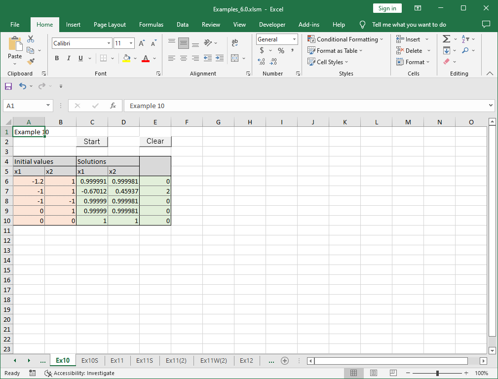
Some initial values, like (-1, 1), failed to converge.

10.3.2 Solving Using VBA Program (2)

Below is an example using Optif0_r, the reverse communication version (RCI).

Sub Start()
    Const NMax = 10, Ndata = 5
    Dim N As Long, X(NMax) As Double, Xpls(NMax) As Double, Fpls As Double
    Dim Info As Long, I As Long
    Dim XX(NMax - 1) As Double, YY As Double, IRev As Long
    N = 2
    For I = 0 To Ndata - 1
        '--- Input data
        X(0) = Cells(6 + I, 1): X(1) = Cells(6 + I, 2)
        '--- Find min point of equation
        IRev = 0
        Do
            Call Optif0_r(N, X(), Xpls(), Fpls, Info, XX(), YY, IRev)
            If IRev = 1 Then YY = 100 * (XX(1) - XX(0) ^ 2) ^ 2 + (1 - XX(0)) ^ 2
        Loop While IRev <> 0
        '--- Output result
        Cells(6 + I, 3) = Xpls(0): Cells(6 + I, 4) = Xpls(1): Cells(6 + I, 5) = Info
    Next
End Sub

Instead of using an external function, this version directly computes function values when IRev = 1, assigns them to YY, and re-calls Optif0_r. More details on RCI are available here.

Running this program produced the same results.

10.3.3 Solving Using the Solver

The XLPack Solver Add-in can also solve the optimization problem using the “Multivariate Nonlinear Optimization” function. The formula (=100*(C8-B8^2)^2+(1-B8)^2) is entered in cell B9.

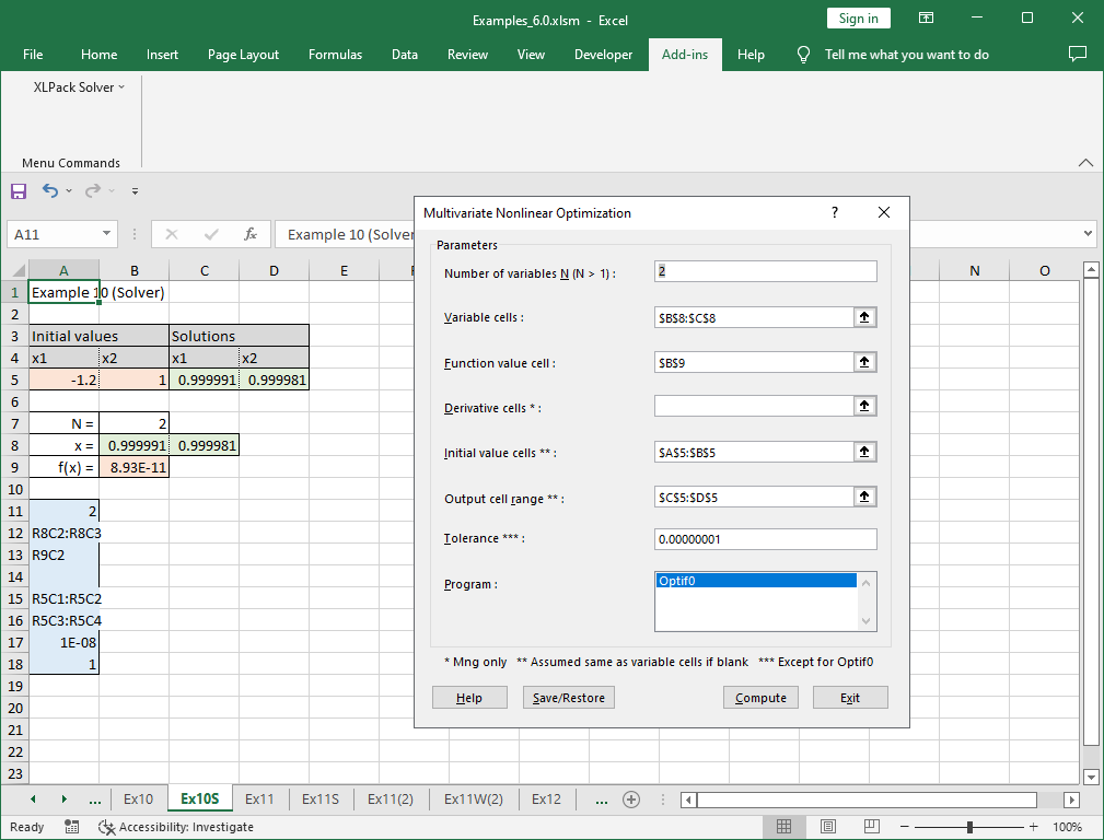
For more information about the solver, refer to this link.