2. Systems of Linear Equations
Note – This document was created using AI translation.2.1 Overview
For example, a system of linear equations with two unknowns (a two-variable system of linear equations) is given as follows.
\[
a_{11}x_1 + a_{12}x_2 = b_1 \\
a_{21}x_1 + a_{22}x_2 = b_2 \\
\]
\(x_1\) and \(x_2\) are the unknowns.
This system can be represented using matrices as follows:
\[
\boldsymbol{A}\boldsymbol{x} = \boldsymbol{b}
\]
Where,
\[
\boldsymbol{A} =
\begin{pmatrix}
a_{11} & a_{12} \\
a_{21} & a_{22} \\
\end{pmatrix},
\boldsymbol{b} =
\begin{pmatrix}
b_1 \\
b_2 \\
\end{pmatrix},
\boldsymbol{x} =
\begin{pmatrix}
x_1 \\
x_2 \\
\end{pmatrix}
\]
The matrix \(\boldsymbol{A}\) is called the coefficient matrix, \(\boldsymbol{b}\) is the right-hand side vector, and \(\boldsymbol{x}\) is the solution vector. The matrix notation remains the same for systems with n unknowns.
If the inverse matrix \(\boldsymbol{A^{-1}}\) is known, multiplying both sides of the equation from the left by it gives:
\[
\boldsymbol{A^{-1}Ax = A^{-1}b}
\]
Since \(\boldsymbol{A^{-1}A}\) cancels out, the solution vector \(\boldsymbol{x}\) can be obtained as:
\[
\boldsymbol{x} = \boldsymbol{A^{-1}}\boldsymbol{b}
\]
Excel provides the worksheet function MINVERSE to calculate the inverse matrix. By using this function to compute \(\boldsymbol{A^{-1}A}\) and multiplying it from the left with the right-hand side vector \(\boldsymbol{b}\), the solution vector \(\boldsymbol{x}\) can be found. However, this method is computationally expensive and may suffer from numerical accuracy issues. Therefore, direct computation without obtaining the inverse matrix is often preferred.
2.1 Solution Methods for Systems of Linear Equations
The general method for solving systems of linear equations on a computer is essentially the same as manual calculations. That is, one equation is multiplied by a constant and subtracted from another, progressively eliminating variables one by one. This process is known as Gaussian elimination.
Expressing this process in matrix form corresponds to decomposing the coefficient matrix into the product of triangular matrices. Systems of linear equations with triangular matrices as coefficients can be easily solved using substitution operations.
2.1.1 General Matrices
First, the coefficient matrix \(\boldsymbol{A}\) is decomposed as follows. This is called LU decomposition.
\[
\boldsymbol{A} = \boldsymbol{LU}
\]
where \(\boldsymbol{L}\) is a lower triangular matrix, and \(\boldsymbol{U}\) is an upper triangular matrix.
There are several variations in LU decomposition procedures, but they are fundamentally based on Gaussian elimination. This process is referred to as forward elimination.
If a diagonal element becomes zero during LU decomposition, calculations cannot proceed. In such cases, swapping the current row with another row where the diagonal element is nonzero allows the process to continue. To minimize numerical errors, swapping with the row containing the largest diagonal element is often preferred. This process is called pivot selection. There are various pivot selection strategies.
Next, we set \(\boldsymbol{y} = \boldsymbol{Ux}\), then solve for \(\boldsymbol{y}\) from \(\boldsymbol{Ly} = \boldsymbol{b}\), and finally determine \(\boldsymbol{x}\) from \(\boldsymbol{Ux} = \boldsymbol{y}\). Since \(\boldsymbol{L}\) and \(\boldsymbol{U}\) are triangular matrices, solutions can be computed easily using substitution operations. This step is called back-substitution.
\[
\begin{align}
&\boldsymbol{LUx} = \boldsymbol{b} \\
&\boldsymbol{Ly} = \boldsymbol{b} \\
&\boldsymbol{Ux} = \boldsymbol{y} \\
\end{align}
\]
By separating the decomposition (forward elimination) from solution computation (back-substitution), the same coefficient matrix can be reused for different right-hand sides, requiring only back-substitution to obtain the solutions.
2.1.2 Symmetric Matrices
The coefficient matrix \(\boldsymbol{A}\) can be decomposed as follows. This is known as Cholesky decomposition.
\[
\boldsymbol{A} = \boldsymbol{LL^T} or \boldsymbol{A} = \boldsymbol{U^TU}
\]
where \(\boldsymbol{L}\) is a lower triangular matrix, and \(\boldsymbol{U}\) is an upper triangular matrix.
The Cholesky decomposition procedure is similar to LU decomposition. However, symmetric matrices that cause diagonal elements to become zero rarely appear in practical applications, so pivot selection is typically not performed.
Once decomposition is complete, the solution is obtained using substitution operations, just like in the case of general matrices.
2.1.3 Condition Number
Evaluating the condition number of the coefficient matrix can provide useful insights when solving systems of linear equations.
The condition number is defined as follows:
\[
cond(\boldsymbol{A}) = ||\boldsymbol{A}||\cdot||\boldsymbol{A^{-1}}||
\]
The condition number ranges from 1 (ideal case, identity matrix \(\boldsymbol{I}\)) to \(\infty\) (worst-case, singular matrix). Typically, its value falls in between. Since computing the condition number directly requires determining the inverse matrix?an expensive operation?simplified estimations are often used.
Using the condition number, the relative error of the computed solution \(\boldsymbol{x}\) can be estimated as:
\[
||\boldsymbol{x^*} – \boldsymbol{x}||/||\boldsymbol{x}|| \leq cond(\boldsymbol{A})\cdot \epsilon
\]
where \(\boldsymbol{x^*}\) is the true solution, and \(\epsilon\) represents machine epsilon (*). When the condition number is excessively large, the system is considered ill-conditioned. For instance, if the condition number is about \(10^{15}\), the solution might contain almost no significant digits.
(*) Machine epsilon refers to the rounding error introduced by representing real numbers in floating-point format. In Excel (IEEE double precision), its approximate value is \(1.11 \times 10^{-16}\).
2.2 Solving Systems of Linear Equations Using XLPack
The VBA subroutines for LU decomposition and Cholesky decomposition in XLPack are Dgesv and Dposv, respectively. The corresponding worksheet functions are WDgesv and WDposv.
To estimate the condition number in a VBA program, the functions Dlange, Dgecon, Dlansy, and Dpocon can be used. In worksheet functions, WDgesv and WDposv also return an estimate of the condition number as part of their results.
These functions utilize subroutines from the LAPACK linear algebra library, including DGESV, DLANGE, DGECON (LU decomposition) and DPOSV, DLANSY, DPOCON (Cholesky decomposition).
Example Problem
Solve the following system of linear equations:
\[
\begin{align}
& 10x_1 – 7x_2 = 7 \\
& -3x_1 + 2x_2 + 6x_3 = 4 \\
& 5x_1 – x_2 + 5x_3 = 6 \\
\end{align}
\]
Expressing this in matrix form:
\[
\boldsymbol{A}\boldsymbol{x} = \boldsymbol{b}
\]
where:
\[
\boldsymbol{A} =
\begin{pmatrix}
10 & -7 & 0 \\
-3 & 2 & 6 \\
5 & -1 & 5 \\
\end{pmatrix},
\boldsymbol{b} =
\begin{pmatrix}
7 \\
4 \\
6 \\
\end{pmatrix},
\boldsymbol{x} =
\begin{pmatrix}
x_1 \\
x_2 \\
x_3 \\
\end{pmatrix}
\]
Here, \(\boldsymbol{A}\) is the coefficient matrix, \(\boldsymbol{b}\) is the right-hand side vector, and \(\boldsymbol{x}\) is the solution vector.
2.2.1 Solving Using Worksheet Functions
First, enter the coefficient matrix \(\boldsymbol{A}\) and right-hand side vector \(\boldsymbol{b}\) into appropriate worksheet cells (orange cells). Then, select a range of cells (solution elements + 2) to enter the worksheet function WDgesv (green cells).
Enter the required parameters (N, A, B, Nrhs) for WDgesv.
N: Number of elements (3 in this example)
A: Cell range of coefficient matrix \(\boldsymbol{A}\)
B: Cell range of right-hand side vector \(\boldsymbol{b}\)
Nrhs: Number of right-hand-side vectors (used when solving for multiple \(\boldsymbol{b}\) values; defaults is 1 if omitted).
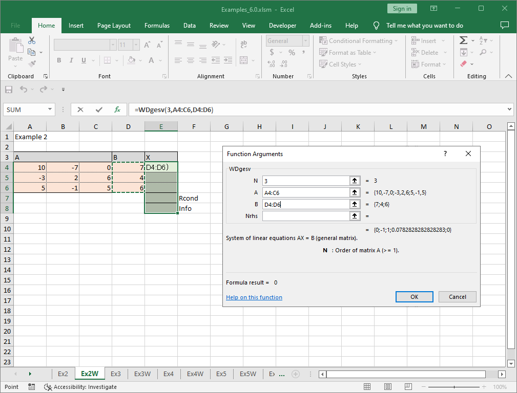
Once input is complete, press Ctrl + Shift + Enter to execute.
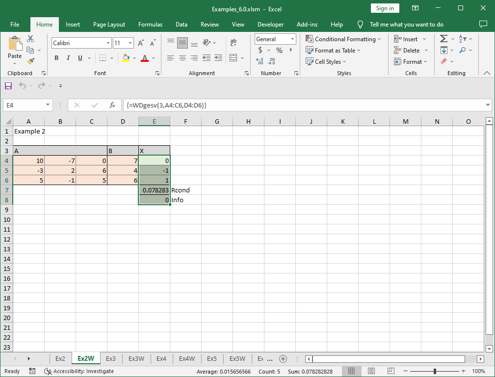
This yields the solution \(\boldsymbol{x} = \begin{pmatrix} 0 & -1 & 1\end{pmatrix}^T\). The displayed 0.078283 is the reciprocal of the estimated condition number, and the 0 at the bottom indicates normal completion (successful execution).
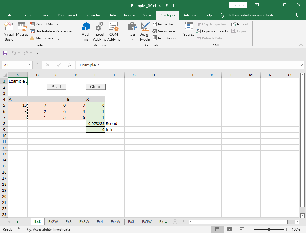
2.2.2 Solving Using VBA Program
The same example can be solved using a VBA program with Dgesv. Here’s a sample implementation:
Sub Start()
    Const NMax = 10
    Dim N As Long, A(NMax, NMax) As Double, B(NMax) As Double
    Dim Anorm As Double, RCond As Double
    Dim Ipiv(NMax) As Long, Info As Long, I As Long, J As Long
    '--- Input data
    N = 3
    For I = 0 To N - 1
        For J = 0 To N - 1
            A(I, J) = Cells(5 + I, 1 + J)
        Next
        B(I) = Cells(5 + I, 4)
    Next
    '--- Solve equation
    Anorm = Dlange("1", N, N, A())
    Call Dgesv(N, A(), Ipiv(), B(), Info)
    If Info = 0 Then
        '--- Compute condition number
        Call Dgecon("1", N, A(), Anorm, RCond, Info)
    End If
    '--- Output solution
    For I = 0 To N - 1
        Cells(5 + I, 5) = B(I)
    Next
    Cells(8, 5) = RCond
    Cells(9, 5) = Info
End Sub
The functions Dlange and Dgecon compute the condition number but are not required for solving the equation itself.
Entering the coefficient matrix \(\boldsymbol{A}\) and right-hand side vector \(\boldsymbol{b}\) into designated worksheet cells (orange cells), then running the macro Start, produces the solution. Unlike the worksheet function approach, the results are not obtained immediately after data entry; execution of the VBA program is necessary.
2.2.3 Handling Symmetric Matrices
For positive definite symmetric matrices, WDposv and Dposv offer a more efficient solution. The procedure is the same as above, except that only the upper or lower triangular portion of A (including diagonal elements) needs to be defined. The remaining portion will be ignored.
Although not included here, the downloadable sample worksheet contains examples using WDposv and Dposv.

