4. Linear Least Squares Method

Note – This document was created using AI translation.

4.1 Overview

Given m measurement data points:

  
  (xi, yi) = (xi + exi, yi + eyi),  i = 1, ..., m

 
where each data point (x_i, y_i) includes measurement errors (e_xi および e_yi) relative to the true values (x_i, y_i).

The true values satisfy a certain function:

  
  yi = F(xi)

 
This function F(x) is approximated using a linear combination of n basis functions φ_j:

  
  F(x) ≒ f(x) = c1φ1(x) + c2φ2(x) + ... + cnφn(x)

 
where f(x) is called the model function. When the number of data points is sufficiently large (m ≫ n), we determine parameters c_j (j=1～n) such that the model function fits the data as accurately as possible.

One commonly used basis function φ_j is:

  
  φj(x) = xj-1

 
which corresponds to polynomial approximation:

  
  f(x) = c1 + c2x + ... + cnxn-1

 
Other approximations that can be expressed as a linear combination can be treated similarly. Examples include:

Trigonometric function approximation:

  
  f(x) = c1sin(x) + c2sin(2x) + ... + cnsin(nx)

 
Exponential function approximation (where \( \lambda_j \) are constants):

  
  f(x) = c1exp(λ1x) + c2exp(λ2x) + ... + cnexp(λnx)

 
Substituting m measurement data points into the model function leads to the following system of linear equations, called the observation equation:

  
  Ac = y

 
where:
– A is an m x n coefficient matrix with elements A_ij = φ_j(x_i) (i = 1～m, j = 1～n).
– c is an n-dimensional solution vector, with elements representing parameters c_j (j=1～n).
– y is an m-dimensional right-hand-side vector, with elements corresponding to measurement data y_i (i=1～m).

Since the number of equations exceeds the number of unknowns (m > n), an exact solution is not possible, and an approximate solution must be obtained. One approach is to minimize the squared norm ||Ac – y||² (*), which leads to the least squares method. The solution c obtained is called the least squares solution.

(*) That is, minimizing the sum of squared residuals Σr_i² where r_i = f(x_i) – y_i for 1 ～ m.

4.2 Linear Least Squares Method

The least squares solution minimizes ||Ac – y||² and satisfies the following equation:

  
  ATAc = ATy

 
This equation, called the normal equation, has n unknowns and n equations, making it solvable. However, the condition number of the coefficient matrix satisfies Cond(A^TA) = (Cond(A))², which can result in large numerical errors. Therefore, this approach is not recommended.

Instead, QR decomposition is widely used. QR decomposition expresses A as:

  
  A = QR

 
where:
– Q is an m x m orthogonal matrix (Q^TQ = I).
– R is an m x n upper triangular matrix, where rows n+1 to m are zero.

Using QR decomposition, the original system of linear equations transforms as follows:

 
  Ac = y
  QRc = y
  QTQRc = QTy
  Rc = QTy

 
Since R is an upper triangular matrix, solving for c requires only substitution, making it straightforward. The resulting c is the least squares solution.

Regarding the choice of parameter count n, increasing it arbitrarily does not necessarily improve the results. For example, fitting a second-degree polynomial to data that clearly follows a linear trend is unnecessary. If n is too large, the columns of A may become linearly dependent, causing the QR decomposition to fail. This is called rank deficiency (rank refers to the number of linearly independent columns). In such cases, it is necessary to reconsider the model function.

4.3 Solving Linear Least Squares Using XLPack

The VBA subroutine Dgels or the worksheet function WDgels can be used to efficiently compute the least squares solution.

These functions utilize the LAPACK subroutine DGELS, which determines the least squares solution using QR decomposition. However, rank deficiency must not be present.

—

Example Problem: Polynomial Approximation

The following data comes from the National Institute of Standards and Technology (NIST) website (http://www.itl.nist.gov/div898/strd/lls/data/Norris.shtml).

 
     y          x
    0.1        0.2
  338.8      337.4
  118.1      118.2
  888.0      884.6
    9.2       10.1
  228.1      226.5
  668.5      666.3
  998.5      996.3
  449.1      448.6
  778.9      777.0
  559.2      558.2
    0.3        0.4
    0.1        0.6
  778.1      775.5
  668.8      666.9
  339.3      338.0
  448.9      447.5
   10.8       11.6
  557.7      556.0
  228.3      228.1
  998.0      995.8
  888.8      887.6
  119.6      120.2
    0.3        0.3
    0.6        0.3
  557.6      556.8
  339.3      339.1
  888.0      887.2
  998.5      999.0
  778.9      779.0
   10.2       11.1
  117.6      118.3
  228.9      229.2
  668.4      669.1
  449.2      448.9
    0.2        0.5

 
This data is approximated using a first-degree polynomial (linear function):

 
  f(x) = c1 + c2x

4.3.1 Solving Using a Worksheet Function

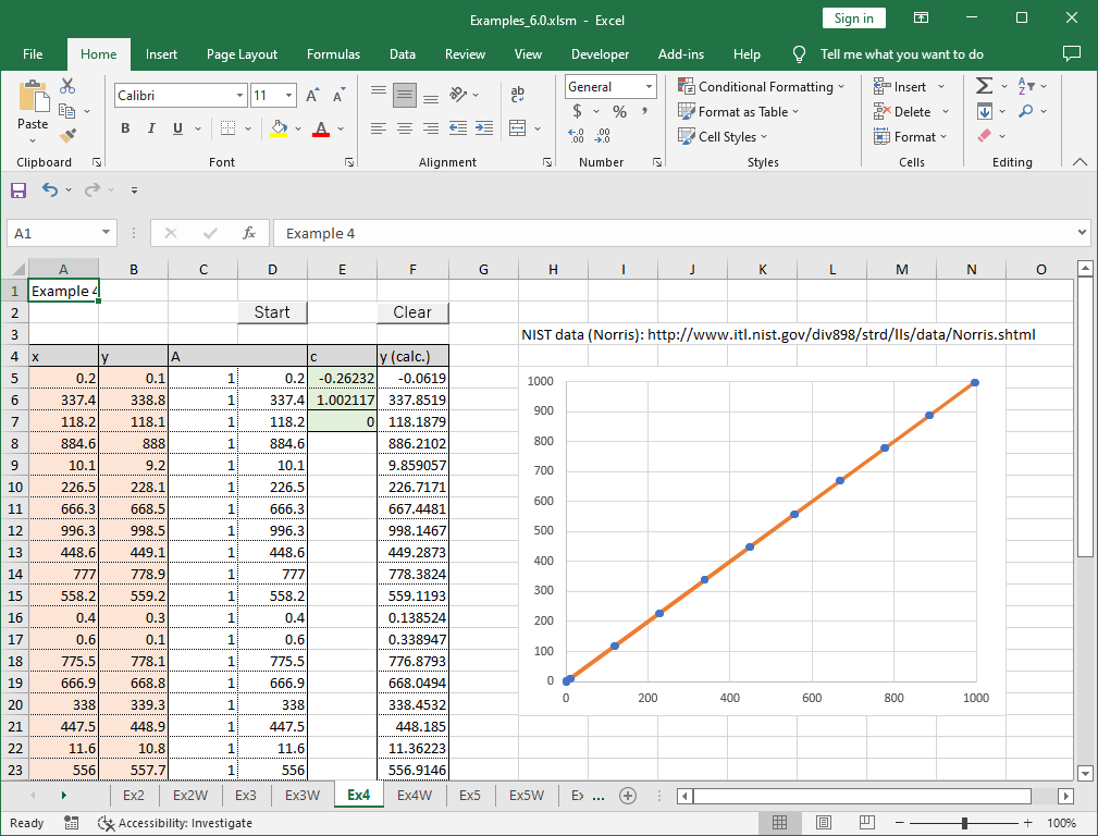
1. Enter the measurement data in an appropriate location in the worksheet (orange-colored cells).

2. Construct the coefficient matrix A where (A_ij = φ_j(x_i) (i = 1～m, j = 1～n)). In this case, A_i1 = 1, and A_i2 = x_i (i = 1～m).

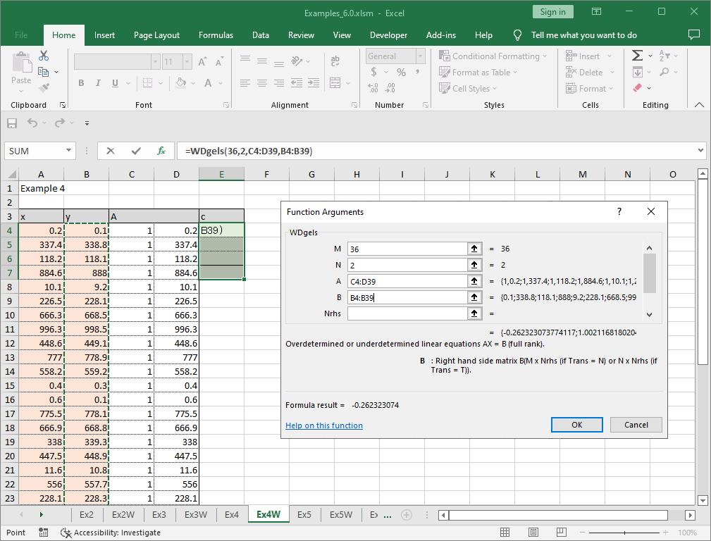
3. Select (n + 2) cells to store the computed parameters c and additional results, and set the worksheet function WDgels (green-colored cells).

Enter the required parameters (Trans, Cov, M, N, A, B, Nrhs) for WDgels.
Trans: “N”: solves Ax = b, “T”: solves A^Tx = b.
Cov: “N”: does not compute the covariance matrix. “D”: computes the variance (diagonal elements of the covariance matrix). “C”: computes the full covariance matrix.
M: Number of data points.
N: Number of parameters (2 in this example).
A: Cell range of matrix A.
B: Cell range of the right-hand-side vector y.
Nrhs: Number of right-hand-side vectors (used when solving for multiple y values; defaults is 1 if omitted).

After entering the function, press Ctrl + Shift + Enter to compute the results. Below is an example visualization where circular markers represent data points, and the computed function is shown as a straight line.

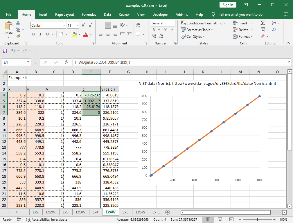
The parameters obtained are c₁ = -0.26232 and c₂ = 1.002117. These match the reference values provided by NIST.

4.3.2 Solving Using a VBA Program

The same problem can be solved using a VBA program with Dgels. Below is an example:

Sub Start()
    Const MMax = 100, NMax = 5
    Dim M As Long, N As Long
    Dim A(MMax, NMax) As Double, B(MMax) As Double
    Dim Info As Long, I As Long, J As Long
    '--- Input data
    M = 36: N = 2
    For I = 0 To M - 1
        For J = 0 To N - 1
            A(I, J) = Cells(5 + I, 3 + J)
        Next
        B(I) = Cells(5 + I, 2)
    Next
    '--- Compute least squares solution
    Call Dgels("N", M, N, A(), B(), Info)
    '--- Output result
    For J = 0 To N - 1
        Cells(5 + J, 5) = B(J)
    Next
    Cells(7, 5) = Info
End Sub

By entering the data in the designated location and running the Start macro, you will obtain the same results as above. Unlike using the worksheet function, simply entering the values for the coefficient matrix A and the right-hand-side vector b does not produce the results. You must execute the VBA program to perform the computation.