5. Interpolation
Note – This document was created using AI translation.5.1 Overview
Interpolation is often confused with the least squares method. In the least squares method, errors in the data points are assumed, meaning the approximation does not pass precisely through the given data points. However, interpolation is a method that smoothly connects data points without errors, ensuring that the interpolation function passes exactly through all given data points. If errors exist in the data points, the resulting interpolation curve may appear unnaturally distorted.
There are numerical tables that list function values for various points. In the past, interpolation was used to estimate values for points not listed in the table. Today, with the availability of scientific calculators and computers, the need for such tables has diminished. However, interpolation is still useful when rapid function evaluation is needed, especially for functions where each computation requires significant effort or time.
Additionally, interpolation serves as a foundational technique in numerical analysis. For example, in numerical integration, interpolation functions of partition points are determined, and the integrated function value of the interpolation function is used as the integral result.
5.2 Solution Methods for Interpolation
5.2.1 Polynomial Interpolation (Lagrange Interpolation)
An \(n\)-th degree polynomial \(p_n(x)\) is defined as follows:
\[
p_n(x) = a_0x^n + a_1x^{n-1} + \dots + a_{n-1}x + a_n
\]
Let’s \(p_n(x)\) be used to interpolate \(f(x)\).
Given function values \(f(x_0), f(x_1), \dots, f(x_n)\) at \(n + 1\) distinct points \(x_0, x_1, \dots, x_n\), the coefficients \(a_0, a_1, \dots, a_n\) can be determined by solving an \((n + 1)\)-variable system of linear equations.
A direct approach to polynomial interpolation involves solving simultaneous linear equations to compute polynomial coefficients. However, in practical applications, the condition number of these equations tends to be high, leading to computational difficulties. Instead, the equivalent polynomial representation known as the Lagrange interpolation formula is often used.
The Lagrange interpolation formula is given by:
\[
f(x) = \sum_{k=0}^{n}L_k(x) f(x_k)
\]
where
\[
L_k(x) = \prod_{i=0}^{n (i \neq k)}(x – x_i)/(x_k – x_i)
\]
The function \(L_k(x_i)\) evaluates to \(1\) when \(i = k\) and \(0\) otherwise. Consequently, the Lagrange interpolation formula ensures the interpolated function matches the given data at each sample point. Furthermore, the order of sample points does not affect the interpolation, and uniform spacing between the points is not required.
Since the Lagrange interpolation formula results in an \(n\)-th degree polynomial, its coefficients match those obtained from solving the system of linear equations. However, in interpolation, obtaining function values is the primary goal rather than determining polynomial coefficients, so the formula is directly used for calculations.
5.2.2 Cubic Spline Interpolation
A method that divides the entire interval into small segments and applies polynomial interpolation to each segment is called piecewise polynomial interpolation. The most commonly used method in this category is cubic spline interpolation. It approximates consecutive data points with cubic polynomials, ensuring smooth connections by enforcing continuity in first and second derivatives at segment boundaries.
Consider data points \((x_1, y_1), (x_2, y_2), \dots, (x_n, y_n)\), referred to as nodes. Cubic splines apply cubic polynomials within the interval \([x_1, x_n]\), ensuring first and second derivative continuity between adjacent segments.
Defining \(n – 1\) cubic polynomials requires four parameters for each segment, necessitating a total of \(4 \times (n – 1)\) parameters. Given \(n\) predetermined values \(y_i\) at the nodes and enforcing continuity of function values, first derivatives, and second derivatives at \(n – 2\) interior nodes (providing \(3 \times (n – 2)\) conditions), we obtain \(4n – 6\) constraints, leaving two degrees of freedom.
To establish the remaining two conditions, known derivatives at \(x_1\) and \(x_n\) can be incorporated. If unavailable, setting the second derivative to zero at \(x_1\) and \(x_n\) defines a natural spline. Alternatively, enforcing continuity of the third derivative at \(x_1\) and \(x_n\) establishes the not-a-knot condition.
Determining these parameters reduces to solving a system of linear equations with a symmetric positive-definite tridiagonal matrix.
5.3 Using XLPack for Interpolation
To compute cubic spline interpolation coefficients, use Pchse, and to evaluate interpolated values, use Pchfe. In spreadsheet functions, WPchse and WPchfe serve the same purpose.
Example: Logarithm Table
The following table is an excerpt from a natural logarithm table:
| n | ln(n) |
|---|---|
| 1.5 | 0.405465108108164 |
| 1.6 | 0.470003629245736 |
| 1.7 | 0.53062825106217 |
| 1.8 | 0.587786664902119 |
| 1.9 | 0.641853886172395 |
| 2.0 | 0.693147180559945 |
| 2.1 | 0.741937344729377 |
| 2.2 | 0.78845736036427 |
5.3.1 Using Worksheet Functions
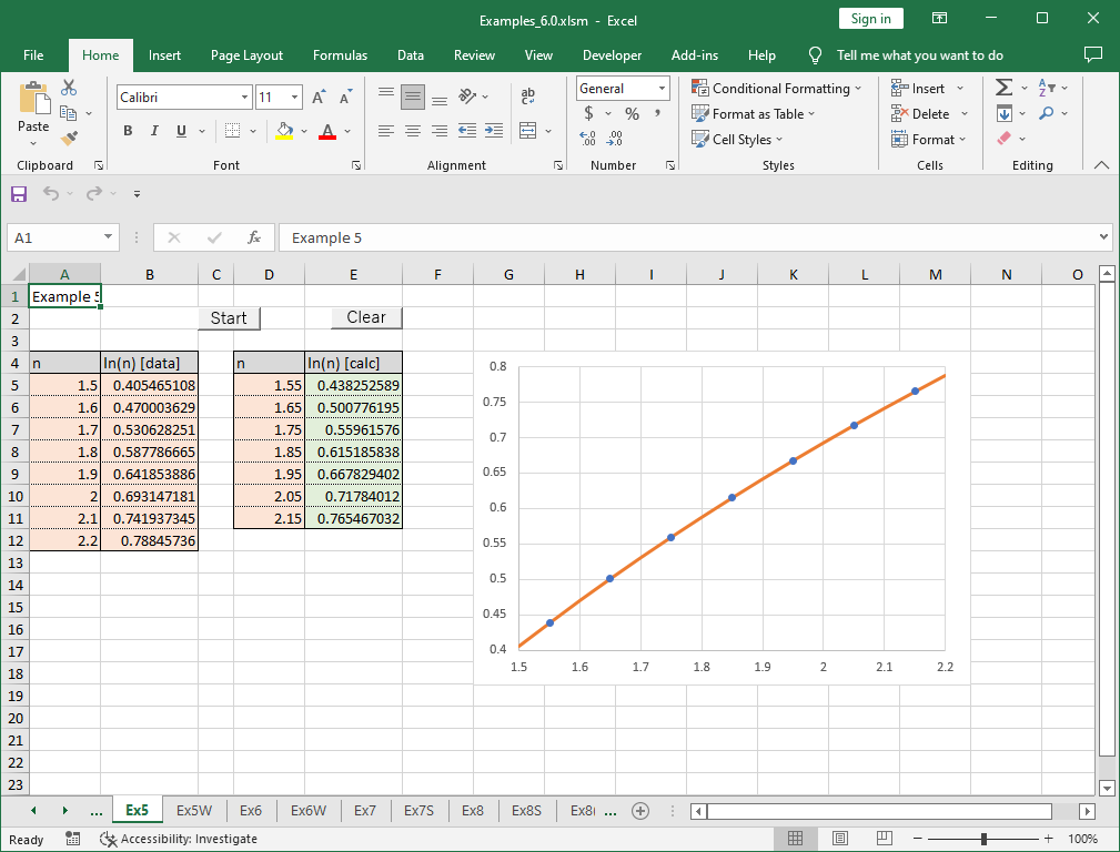
First, enter the data points \((x_i, y_i = ln(x_i))\) into an appropriate section of the worksheet (orange-colored cells on the left). The \(x_i\) values must be in ascending order. Then, select a range of cells and use the worksheet function WPchse to compute the spline interpolation coefficients \(d_i\) (green-colored cells on the left).
The required parameters for WPchse are N, X and Y. N is the number of data points (8 in this example). X and Y are the cell ranges containing the interpolation data \((x_i, y_i)\).
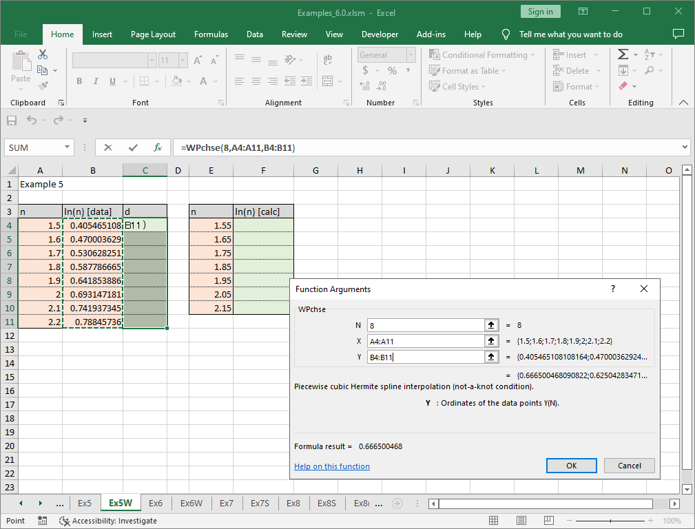
After inputting the values, press Ctrl + Shift + Enter. The spline interpolation coefficients are now determined.
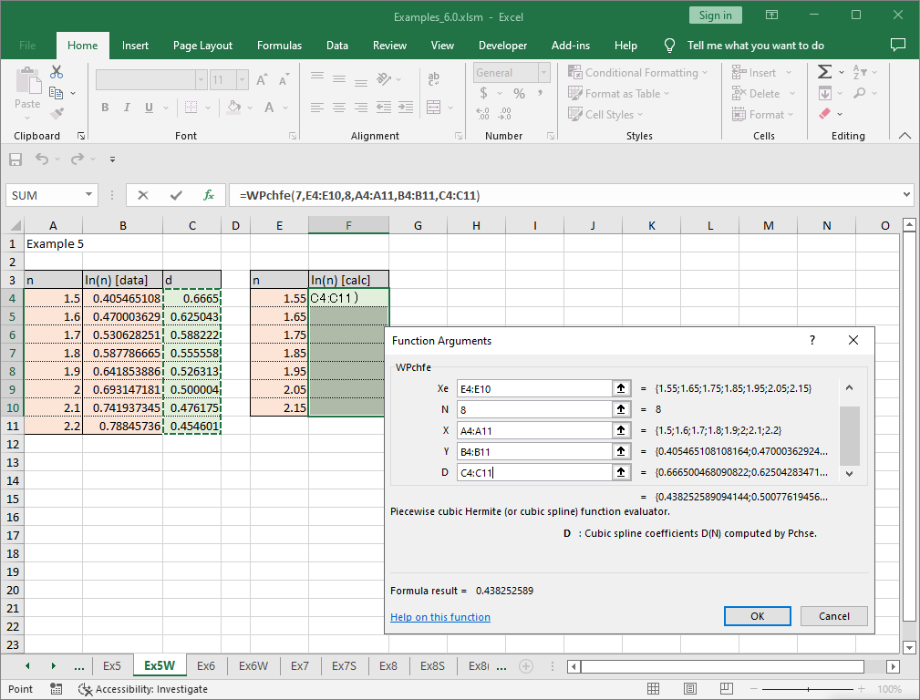
Next, enter the points where you want to compute values (in this case, \(n = 1.55 \sim 2.15\)) into another section (orange-colored cells on the right). Use the worksheet function WPchfe to compute function values at those points (green-colored cells on the right).
The required parameters for WPchfe are Ne, Xe, N, X, Y and D. Ne is the number of points to interpolate (7 in this example). Xe is the cell range containing the points to be evaluated. N, X and Y are the same data used for WPchse. D is the computed interpolation coefficients.
Press Ctrl + Shift + Enter to compute the natural logarithm values at the points not included in the table. The plot below shows the given table values as a solid line and interpolated values as circles.
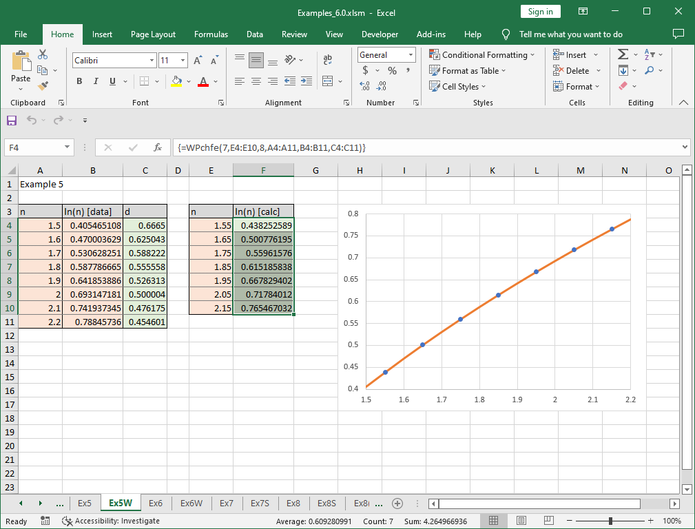
In this example, the data points are evenly spaced, but this is not a requirement. However, interpolation accuracy decreases in intervals where data points are sparsely distributed. Additionally, extrapolated values (outside the given data range) can be computed but tend to have lower precision.
5.3.2 Using VBA Programming
The same example can be solved using a VBA program. Below is an example using Pchse and Pchfe.
Sub Start()
    Const NMax = 10
    Dim N As Long, Ne As Long, I As Long, Info As Long
    Dim X(NMax) As Double, Y(NMax) As Double, D(NMax) As Double
    Dim Xe(NMax) As Double, Fe(NMax) As Double
    '--- Input data
    N = 8
    For I = 0 To N - 1
        X(I) = Cells(5 + I, 1)
        Y(I) = Cells(5 + I, 2)
    Next
    '--- Compute coefficients of a cubic spline
    Call Pchse(N, X(), Y(), D(), Info)
    If Info <> 0 Then
        MsgBox "** Error in Pchse **  Info = " + Str(Info)
        Exit Sub
    End If
    '--- Compute interpolated values
    Ne = N - 1
    For I = 0 To Ne - 1
        Xe(I) = Cells(5 + I, 4)
    Next
    Call Pchfe(N, X(), Y(), D(), Ne, Xe(), Fe(), Info)
    If Info <> 0 Then
        MsgBox "** Error in Pchfe **  Info = " + Str(Info)
        Exit Sub
    End If
    '--- Output result
    For I = 0 To Ne - 1
        Cells(5 + I, 5) = Fe(I)
    Next
End Sub
After entering the data in the designated location (orange-colored cells), run the macro Start to obtain results. Unlike the worksheet function method, results are not immediately computed upon entering interpolation data – you must execute the VBA program.