6. Algebraic Equations

6.1 Overview

An algebraic equation is a problem of finding the zeros of a polynomial function:
\[
p(x) = a_0x^n + a_1x^{n-1} + \dots + a_{n-1}x + a_n = 0
\] As is well known, quadratic, cubic, and quartic equations can be solved using formulaic solutions. For equations of degree five or higher (high-degree algebraic equations), numerical methods (iterative techniques) are generally required. Even for cubic and quartic equations, numerical methods may sometimes be preferable.

6.2 Solving High-Degree Algebraic Equations

Many methods have been proposed to solve high-degree algebraic equations, such as Bairstow’s method, Graeffe’s method, Bernoulli’s method, and Jenkins-Traub’s method. However, no single method has emerged as the definitive approach.

If only one specific root needs to be found, Newton’s method can be used as a numerical method for solving nonlinear equations (see Chapter 7). However, a good initial estimate is necessary.

To determine all roots, the following methods can be employed:

6.2.1 Simultaneous Method

This is an iterative approach that determines all roots simultaneously.

Representing the \(k\)-th iterative approximation as superscript \((k)\), Newton’s method for computing each root uses the following recurrence relation:
\[
x_i^{(k+1)} = x_i^{(k)} – p(x_i^{(k)})/p'(x_i^{(k)})
\] Approximating \(p'(x_i^{(k)})\) as \(\prod_{j=1}^{n, j \neq i}(x_i^{(k)} – x_j^{(k)})\), the recurrence equation becomes as follows.
\[
x_i^{(k+1)} = x_i^{(k)} – p(x_i^{(k)})/\prod_{j=1}^{n, j \neq i}(x_i^{(k)} – x_j^{(k)})
\] This is called the simultaneous method (second-order method) and converges quadratically if there are no multiple roots. It is also known as the Durand-Kerner method.

Thereare various initialization and approximation techniques. Some modifications increase computational effort but achieve cubic convergence for non-multiple roots, referred to as third-order methods. A variant using Aberth’s proposed initial values is known as the Durand-Kerner-Aberth (DKA) method.

6.2.2 Companion Matrix Method

In eigenvalue problems, explanations often state that “The characteristic equation associated with eigenvalue \(\lambda\) is an \(n\)-th degree algebraic equation, and solving it yields the eigenvalues”. However, in practice, solving the algebraic equation directly is more challenging. Instead, a companion matrix is constructed corresponding to the given algebraic equation, and the eigenvalues of this matrix are determined using QR decomposition or other eigenvalue-solving techniques. This indirectly provides the solutions to the algebraic equation.

6.3 Solving Algebraic Equations Using XLPack

The VBA subroutine Rpzero2 solves algebraic equations with real coefficients using the simultaneous method (second-order method). It can also determine complex roots. In worksheet functions, WRpzero2 is available for use.

Example Problem

Solve the following fifth-degree equation:
\[
x^5 + 2x^3 + 2x^2 – 15x + 10 = 0
\] Factorizing:
\[
(x – 1)^2(x + 2)(x^2 + 5) = 0
\] This reveals the roots \(1(double root), -2 and \pm\sqrt{5}i\).

6.3.1 Solving Using Worksheet Functions

Enter the polynomial coefficients \(a_i\) into an appropriate section of the worksheet (orange-colored cells). Next, select an \((n + 1) \times 3\) cell range for storing the solutions \((x(r), x(i))\), and error bounds \(s(i)\), then use the worksheet function WRpzero2 (green-colored cells).

The required parameters for WRpzero2 are N and A. N is the degree of the equation (5 in this example). A is the cell range containing the polynomial coefficients. The equation is expressed as \(a_0 x^n + a_1x^{n-1} + \dots + a_{>n-1}x + a_n = 0\) with coefficients represented as real numbers \(a_0, a_1, \dots, a_n\).

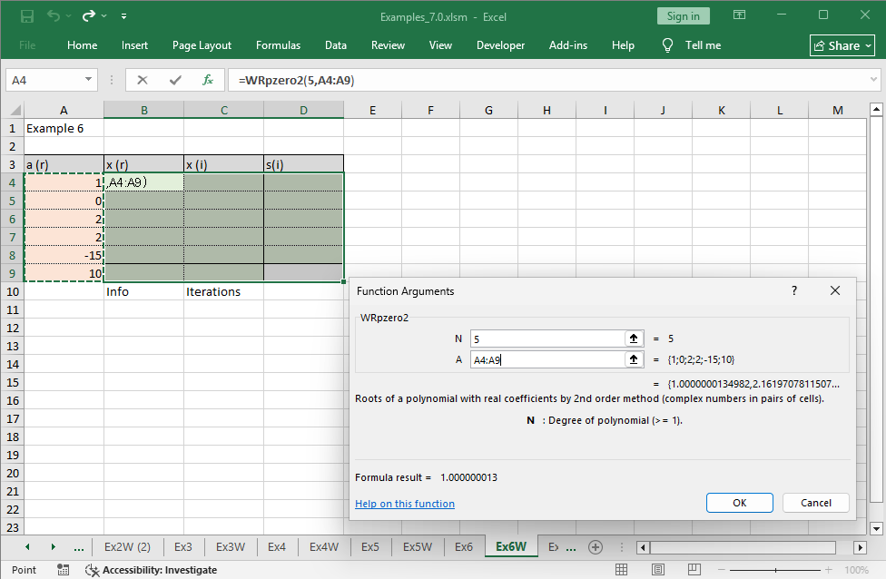
After entering the data, press Ctrl + Shift + Enter.

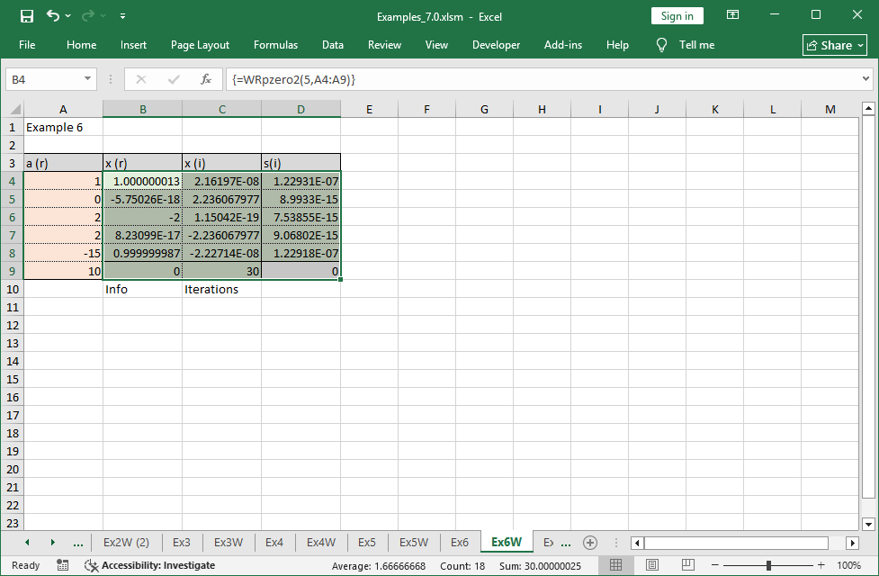
The five solutions have been successfully determined. The rightmost column s(i) represents error bounds, while the bottom row shows return codes and iteration count required for convergence.

For the multiple root \(x = 1\), precision is roughly halved. In numerical computations of algebraic equations, the significant digits of a solution tend to reduce to approximately \(1/m\) for an \(m\)-multiple root, so caution is required.

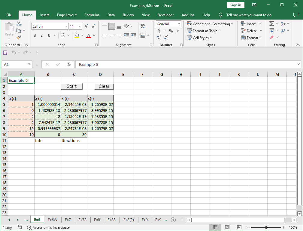
6.3.2 Solving Using VBA Programming

The same example problem is solved using a VBA program. Below is an example of a program that utilizes Rpzero2.

Sub Start()
    Const NMax = 10
    Dim N As Long
    Dim A(NMax) As Double, XR(NMax) As Double, XI(NMax) As Double, S(NMax) As Double
    Dim IFlag As Long, Info As Long, Iter As Long, I As Long
    '--- Input data
    N = 5
    For I = 0 To N
        A(I) = Cells(5 + I, 1)
    Next
    '--- Compute roots of equation
    IFlag = 0
    Call Rpzero2(N, A(), XR(), XI(), IFlag, S(), Info, Iter)
    Cells(10, 2) = Info
    Cells(10, 3) = Iter
    '--- Output roots
    For I = 0 To N - 1
        Cells(5 + I, 2) = XR(I)
        Cells(5 + I, 3) = XI(I)
        Cells(5 + I, 4) = S(I)
    Next
End Sub

Enter the coefficient data into the designated location (orange-colored cells), then execute the macro Start to obtain results. Unlike using worksheet functions, simply inputting the coefficient data does not yield results – you must run the VBA program for computations.