Example program of XLPack for Python and XLPack for Matplotlib: (1) 3D visualization (Laplace equation)
We consider solving the following partial differential equation in the square domain \(x = 0 \sim 1, y = 0 \sim 1\).\[
-d^2u/dx^2 – d^2u/dy^2 = 0
\] The boundary conditions are given as follows.
\[
u(x, 0) = 0, u(0, y) = 0, u(x, 1) = x, u(1, y) = y \space (ディリクレ条件)
\]
Such partial differential equations are applied, for example, to describe the temperature distribution of a plate in thermal equilibrium.
A commonly used method for solving this equation is the finite difference method. For an example of obtaining a numerical solution using the five-point finite difference approximation, see below.
Tutorial for XLPack numerical library: 16. Linear Calculations of Sparse Matrices
Here, we explain an example of obtaining the solution using another method, the finite element method, and visualizing it in 3D.
The square domain is uniformly divided into \(Nx\) and \(Ny\) segments in the \(x\)- and \(y\)-directions, respectively, to form a rectangular grid. Each rectangle is then subdivided into two triangles, thereby generating a simple triangular mesh.
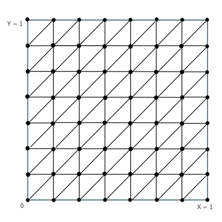
Using this mesh, we obtain the solution by the finite element method. Although the figure above shows an example with 7 divisions (8 x 8 grid), the actual computation was performed with 19 divisions (20 x 20 grid), i.e., (Nx = 19) and (Ny = 19).
1. Overall structure
The main program is as follows.
Sub Main()
    Const Nx = 19, Ny = 19
    Const Nb2 = 0, LdKnc = 4, LdKs = 3
    Const N = (Nx + 1) * (Ny + 1), Ne = 2 * Nx * Ny, Nb = 2 * (Nx + Ny)
    Dim X(N - 1) As Double, Y(N - 1) As Double
    Dim P(N - 1) As Double, Q(N - 1) As Double, F(N - 1) As Double
    Dim Knc(LdKnc - 1, Ne - 1) As Long, Ks(LdKs - 1, Nb - 1) As Long
    Dim Lb(Nb - 1) As Long, Ib(Nb - 1) As Long, Bv(Nb - 1) As Double
    Dim Ks2() As Long, Alpha() As Double, Beta() As Double
    Dim Val(20 * N) As Double, Ptr(N) As Long, Ind(20 * N) As Long
    Dim B(N - 1) As Double, U(N - 1) As Double
    Dim Ux As Double, Err As Double
    Dim Info As Long
    Dim I As Long, J As Long
    '-- Set mesh data
    Call SetData(Nx, Ny, N, Ne, Nb, X(), Y(), Knc(), Ks(), Lb(), P(), Q(), F(), Ib(), Bv())
    '-- Assemble FEM matrix
    Call Fem2p(N, Ne, X(), Y(), Knc(), P(), Q(), F(), Nb, Ib(), Bv(), Nb2, Ks2(), Alpha(), Beta(), Val(), Ptr(), Ind(), B(), Info)
    '-- Solve equation by CG method
    Dim Iter As Long, Res As Double
    Call Cg1(N, Val(), Ptr(), Ind(), B(), U(), Info, Iter, Res)
    Debug.Print "Info =" + Str(Info) + ", Iter =" + Str(Iter) + ", Res =" + Str(Res)
    If Info <> 0 Then Exit Sub
    '-- Plot solution
    Call Plot(Nx, Ny, U())
End Sub
The subroutine Fem2p() in the XLPack library assembles the finite element matrix. This produces a system of equations consisting of a coefficient matrix in sparse (CSR) format and a right-hand-side vector. Since the coefficient matrix is symmetric, the system can be solved by the conjugate gradient method using the subroutine Cg1() in the XLPack library.
The subroutine SetData() sets the data for the grid points, finite elements, and boundary conditions that are used as input to Fem2p().
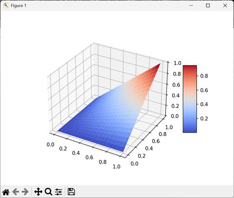
The obtained solution is displayed by the subroutine Plot(). In Plot(), 3D visualization is performed using XLPack for Python or XLPack for Matplotlib.
The execution result will be as follows.
2. Input data settings
A simple triangular mesh can be generated using the subroutine Mesh23() in the XLPack library.
Next, we set the coefficients of the Laplace equation as p(x, y) = 1, q(x, y) = 0, and f(x, y) = 0. We also set the Dirichlet boundary conditions.
The following subroutine performs these tasks.
Sub SetData(Nx As Long, Ny As Long, N As Long, Ne As Long, Nb As Long, X() As Double, Y() As Double, Knc() As Long, Ks() As Long, Lb() As Long, P() As Double, Q() As Double, F() As Double, Ib() As Long, Bv() As Double)
    Dim Id() As Long
    Dim I As Long, J As Long, K As Long
    '-- Generates simple rectangular mesh for 2D triangular element
    Call Mesh23(Nx, Ny, X(), Y(), Knc(), Ks(), Lb())
    '-- Set p(x, y) = 1, q(x, y) = 0 and f(x, y) = 0
    For I = 0 To N - 1
        P(I) = 1
        Q(I) = 0
        F(I) = 0
    Next
    '-- Set boundary condition 1
    ReDim Id(N - 1)
    For I = 0 To Nb - 1
        For J = 1 To 2
            Id(Ks(J, I) - 1) = Lb(I)
        Next
    Next
    K = 0
    For I = 0 To N - 1
        If Id(I) = 1 Or Id(I) = 4 Then
            Bv(K) = 0
        ElseIf Id(I) = 2 Then
            Bv(K) = Y(I)
        ElseIf Id(I) = 3 Then
            Bv(K) = X(I)
        Else
            GoTo Continue
        End If
        Ib(K) = I + 1
        K = K + 1
Continue:
    Next
End Sub
3. 3D visualization of solution
The obtained solution can be visualized using Python code directly written with using XLPack for Python.
Sub Plot(Nx As Long, Ny As Long, U() As Double)
    Dim I As Long
    For I = 0 To (Nx + 1) * (Ny + 1) - 1
        Cells(6 + I, 2) = U(I)
    Next
    '-- Python codes
    PY "import matplotlib.pyplot as plt"
    PY "from matplotlib import cm"
    PY "import numpy as np"
    PY "from XLPackPy import *"
    PY "nx =" + Str(Nx) + "+ 1"
    PY "ny =" + Str(Ny) + "+ 1"
    PY "U = xlc_get(5, 1, 4 + nx*ny)"
    PY "X = np.empty((ny, nx))"
    PY "Y = np.empty((ny, nx))"
    PY "Z = np.empty((ny, nx))"
    PY _
      "for i in range(ny):" + vbNewLine + _
      "  for j in range(nx):" + vbNewLine + _
      "    X[i][j] = (1.0/(nx - 1))*j" + vbNewLine + _
      "    Y[i][j] = (1.0/(ny - 1))*i" + vbNewLine + _
      "    Z[i][j] = U[nx*i + j]"
    PY "fig = plt.figure()"
    PY "ax3 = fig.add_subplot(projection='3d')"
    PY "surf = ax3.plot_surface(X, Y, Z, cmap=cm.coolwarm)"
    PY "fig.colorbar(surf, shrink=0.5, aspect=5)"
    PY "plt.show()"
End Sub
Using XLPack for Matplotlib, everything can be written in VBA. Fig.Add_subplot_3d() corresponds to Python’s fig.add_subplot(projection=’3d’). Except that, the code is almost the same as in Python.
Dim Plt As New Pyplot

Sub Plot(Nx As Long, Ny As Long, U() As Double)
    Dim X() As Double, Y() As Double, Z() As Double
    ReDim X(Ny, Nx), Y(Ny, Nx), Z(Ny, Nx)
    Dim I As Long, J As Long
    Dim Fig As Figure, Ax3 As Axs3d, Surf As PyObject
    '-- Prepare data
    For I = 0 To Ny
        For J = 0 To Nx
            X(I, J) = (1# / Nx) * I
            Y(I, J) = (1# / Ny) * J
            Z(I, J) = U((Nx + 1) * I + J)
        Next
    Next
    '-- Plot by Matplotlib
    Set Fig = Plt.Figure()
    Set Ax3 = Fig.Add_subplot_3d()
    Set Surf = Ax3.Plot_surface(Ny + 1, Nx + 1, X(), Y(), Z(), "coolwarm")
    Call Fig.Colorbar(Surf, KwArgs:="shrink=0.5, aspect=5")
    Call Plt.Show
End Sub
