Example program of XLPack for Python and XLPack for Matplotlib: (2) Animation (Simple pendulum)
As shown in the figure below, consider a mass of weight \(m\) suspended by a string of length \(l\) (whose weight is assumed to be negligible) oscillating from side to side. Let \(\theta\) denote the angle measured from the vertical position of the string. This system is called a simple pendulum.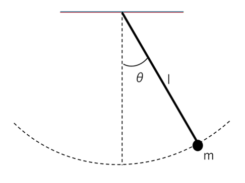
This motion can be described by the following differential equation, where \(t\) denotes time. Here, \(g\) is the acceleration due to gravity \((9.81 m/s^2)\).
\(d^2\theta/dt^2 = -(mg/l)sin\theta\)
For simplicity, we assume \(m = 1\), and compute the numerical solution over the interval \(t = 0 \sim 10\) with the initial conditions \(\theta = \pi/4\) and \(d\theta/dt = 0\). The result will then be displayed as an animation.
1. Overall structure
The main program is as follows.
Sub Main()
    Dim N As Long, T As Double, Y() As Double, Yp() As Double
    Dim Nt As Long, Tend As Double
    Dim X1() As Double, Y1() As Double
    Dim Info As Long
    N = 1
    ReDim Y(N - 1), Yp(N - 1)
    '-- Initial values
    T = 0
    Y(0) = Atn(1)   ' Pi() / 4
    Yp(0) = 0
    '-- Solve ODE
    Tend = 10
    Nt = 200
    ReDim X1(Nt - 1), Y1(Nt - 1)
    Call ODE_2(N, T, Y(), Yp(), Nt, Tend, X1(), Y1(), Info)
    If Info <> 0 Then Exit Sub
    '-- Display animation
    Call Animate(Nt, X1(), Y1(), Tend / Nt)
End Sub
The subroutine ODE_2() solves the differential equation. The obtained solution is displayed by the subroutine Animate(). In Animate(), animation is performed using XLPack for Python or XLPack for Matplotlib.
The execution result will be as follows.
2. Solutions to differential equations
Since the differential equation of a simple pendulum is a second-order ordinary differential equation, it is usually rewritten as the following system of first-order ordinary differential equations before being numerically solved.
\(d\theta_1/dt = \theta_2\)
\(d\theta_2/dt = -(mg/l)sin\theta_1\)
However, in this case, the equation has a special form that does not depend on first-order terms, so it can be solved directly in its original form using the subroutine Dopn43() (Runge-Kutta-Nystrom method) in the XLPack library.
Const L = 1, M = 1, G = 9.81
Const Mode = 3

Sub F_2(N As Long, T As Double, Y() As Double, Ypp() As Double)
    Ypp(0) = -(M * G / L) * Sin(Y(0))
End Sub

Sub ODE_2(N As Long, T As Double, Y() As Double, Yp() As Double, Nt As Long, Tend As Double, X1() As Double, Y1() As Double, Info As Long)
    Dim RTol(0) As Double, ATol(0) As Double
    Dim Dt As Double, Tout As Double, I As Long
    RTol(0) = 0.0000000001 '1e-10
    ATol(0) = RTol(0)
    Dt = Tend / Nt
    Info = 0
    For I = 0 To Nt - 1
        Tout = (I + 1) * Dt
        Call Dopn43(N, AddressOf F_2, T, Y(), Yp(), Tout, Tend, RTol(), ATol(), Mode, Info)
        If Info < 0 Or Info > 10 Then
            MsgBox ("Error in Dopn43: Info =" + Str(Info))
            Exit Sub
        End If
        X1(I) = L * Sin(Y(0))
        Y1(I) = -L * Cos(Y(0))
    Next
End Sub
The obtained solution is converted into XY coordinates and returned in X1() and Y1().
3. Animation of the Solution
The obtained solution can be directly visualized using Python code written with using XLPack for Python.
Since array data cannot be passed directly, the data is first written to a worksheet and then read on the Python side using xlc_get().
Sub Animate(Nt As Long, X1() As Double, Y1() As Double, Dt As Double)
    Dim I As Long
    For I = 0 To Nt - 1
        Cells(6 + I, 2) = X1(I)
        Cells(6 + I, 3) = Y1(I)
    Next
    '-- Python codes
    PY "import matplotlib.pyplot as plt"
    PY "import matplotlib.animation as animation"
    PY "from XLPackPy import *"
    PY "nt =" + Str(Nt)
    PY "dt =" + Str(Dt)
    PY "x1 = xlc_get(5, 1, 4 + nt)"
    PY "y1 = xlc_get(5, 2, 4 + nt)"
    PY "fig = plt.figure()"
    PY "ax = fig.gca()"
    PY "ax.set_xlim(-1.0, 1.0)"
    PY "ax.set_ylim(-1.5, 0.5)"
    PY "ax.set_aspect('equal')"
    PY "ax.grid()"
    PY "ax.set_title('Animation (Pendulum)')"
    PY "xt = []"
    PY "yt = []"
    PY "artist = []"
    PY _
      "for i in range(nt):" + vbNewLine + _
      "  pend, = ax.plot([0, x1[i]], [0, y1[i]], 'o-', color = 'b', lw=2)" + vbNewLine + _
      "  xt.append(x1[i])" + vbNewLine + _
      "  yt.append(y1[i])" + vbNewLine + _
      "  trace, = ax.plot(xt, yt, ':c', lw=1)" + vbNewLine + _
      "  artist.append((pend, trace))"
    PY "anim = animation.ArtistAnimation(fig, artist, interval = dt * 1000)"
    PY "plt.show()"
End Sub
Using XLPack for Matplotlib, the same processing can be written entirely in VBA. Internally, the processing is carried out by calling Python.
Dim Plt As New PyPlot
Dim Animation As New Animation

Sub Animate(Nt As Long, X1() As Double, Y1() As Double, Dt As Double)
    Dim Fig As Figure, Ax As Axs, Artist() As PyObject, Anim As Animation
    Dim X(1) As Double, Y(1) As Double
    Dim I As Long
    ReDim Artist(Nt - 1, 1)
    Set Fig = Plt.Figure()
    Set Ax = Fig.Gca()
    Call Ax.Set_xlim(-1, 1)
    Call Ax.Set_ylim(-1.5, 0.5)
    Call Ax.Set_aspect(1)
    Call Ax.Grid
    Call Ax.Set_title("Animation (Pendulum)")
    X(0) = 0: Y(0) = 0
    For I = 0 To Nt - 1
        X(1) = X1(I): Y(1) = Y1(I)
        Set Artist(I, 0) = Ax.Plot(2, X(), Y(), "o-", "color=b,lw=2")
        Set Artist(I, 1) = Ax.Plot(I + 1, X1(), Y1(), ":c", "lw=1")
    Next
    Set Anim = Animation.ArtistAnimation(Fig, Nt, 2, Artist(), "interval =" + Str(Dt * 1000))
    Call Plt.Show
End Sub
