14. Nonlinear Least Squares Method

Note – This document was created using AI translation.

14.1 Overview

Consider a set of m measurement data points:

  
  (xi, yi) = (x*i + exi, y*i + eyi), i = 1～m

 
where each data point (x_i, y_i) contains measurement errors (e_xi および e_yi) relative to the true values (x^*_i, y^*_i).

Each true value satisfies a function:

  
  y*i = F(x*i)

 
We aim to approximate this function F(x) using a general function f(x), called the model function, which includes n parameters c_j (j = 1 to n):

  
  F(x) ≒ f(x; c) = f(x; c1, c2, ... , cn)

 
One method for determining the n parameters c so that the model function f(x) best fits the data is nonlinear least squares. The parameters c are chosen to minimize the the sum of squared residuals:

  
  Σri2 (i = 1 to m)
  where residual ri = f(xi; c) - yi

14.2 Solution to Nonlinear Least Squares Method

Consider the following function R(x):

  
  R(x) = (1/2)r(x)Tr(x) = Σ(ri(x))2 (i = 1～m)

  where,
         ( r1(x) )
         ( r2(x) )
  r(x) =     ...
         ( rm(x) )

 
The gradient ∇R(x) and the Hessian matrix H(x) of R(x) can be expressed as follows:

  
  ∇R(x) = J(x)Tr(x)
  H(x) = J(x)TJ(x) + S(x)

  where, J(x) is the Jacobian matrix, and S(x) = Σ∂2ri/(∂xk∂xj)ri(x) (Σ for i = 1 to m) (j, k = 1 to n).

 
That is, when applying Newton’s method for nonlinear optimization with R(x) as the objective function, the special structure of R(x), which is the sum of squares of r_i(x), allows the necessary gradient and Hessian matrix in the iterative formula to be derived using the Jacobian matrix.

At this point, using f(x; c) and y from Section 14.1, we redefine r_i as follows:

  
  ri(c) = f(xi; c) - yi, i = 1～m

 
Thus, r_i is considered a function of the parameter c, representing the residuals. With this definition, when solving the nonlinear optimization problem using Newton’s method with R(c) as the objective function, the gradient and Hessian matrix of R(c) can be computed using the Jacobian matrix.

From this point on, we will express c in terms of x and denote it as R(x).

14.2.1 Gauss-Newton Method

We solve the nonlinear optimization problem with R(x) as the objective function using Newton’s method. However, when computing the Hessian matrix, we approximate it by omitting the S(x) term (i.e., assuming S(x) = 0).

With this approximation, the direction vector can be obtained by solving the following system of linear equations:

  
  J(xk)TJ(xk)dk = -J(xk)Tr(xk)

 
This equation is in the form of the normal equations used in linear least squares. Instead of solving it directly, we use methods such as QR decomposition, similar to linear least squares.

14.2.2 Levenberg-Marquardt Method

In the Gauss-Newton method, if the Jacobian matrix loses rank during iteration, the system of linear equations may become unsolvable.

To address this issue, the Levenberg-Marquardt method introduces a parameter λ_k and adds the term λ_kI to ensure that the coefficient matrix remains positive definite:

  
  (J(xk)TJ(xk) + λkI)dk = -J(xk)Tr(xk)

 
If λ_k = 0, the method is identical to the Gauss-Newton method. On the other hand, when λ_k = 0 is large, the algorithm approaches the steepest descent method.

The convergence behavior varies based on the choice of λ_k, and several strategies have been proposed for determining its value.

14.3 Solving Nonlinear Least Squares Using XLPack

The Levenberg-Marquardt method can be implemented using the VBA subroutine Lmdif1. This subroutine calculates derivatives (Jacobian matrix) using finite difference approximation, eliminating the need for users to compute derivatives manually. Lmdif1 can also be accessed from the XLPack solver.

Similar to nonlinear optimization, it is essential to provide an initial value that is as close as possible to the desired solution.

Example Problem

We use test data published on the NIST (National Institute of Standards and Technology) website (https://www.itl.nist.gov/div898/strd/nls/data/misra1a.shtml).

The following model function is used.

  
  f(x) = c1(1 - exp(-c2x))

 
The data is as follows:

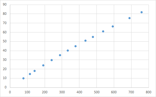
The test data has two specified initial values (500, 0.0001) and (250, 0.0005). The known solutions are c1 = 2.3894212918×10² and c2 = 5.5015643181×10^-4.

14.3.1 Solving Using a VBA Program (1)

Below is an example program using Lmdif1.

Const Ndata = 14, Nparam = 2
Dim Xdata(Ndata - 1) As Double, Ydata(Ndata - 1) As Double

Sub F(M As Long, N As Long, X() As Double, Fvec() As Double, IFlag As Long)
    Dim I As Long
    For I = 0 To M - 1
        Fvec(I) = Ydata(I) - X(0) * (1 - Exp(-Xdata(I) * X(1)))
    Next
End Sub

Sub Start()
    Dim X(Nparam - 1) As Double, Fvec(Ndata - 1) As Double, Tol As Double
    Dim Info As Long, I As Long
    '--- Input data
    For I = 0 To Ndata - 1
        Xdata(I) = Cells(9 + I, 1)
        Ydata(I) = Cells(9 + I, 2)
    Next
    '--- Start calculation
    Tol = 0.0000000001  '** 1e-10
    For I = 0 To 1
        '--- Initial values
        X(0) = Cells(6 + I, 1)
        X(1) = Cells(6 + I, 2)
        '--- Nonlinear least squares
        Call Lmdif1(AddressOf F, Ndata, Nparam, X(), Fvec(), Tol, Info)
        '--- Output result
        Cells(6 + I, 3) = X(0)
        Cells(6 + I, 4) = X(1)
        Cells(6 + I, 5) = Info
    Next
End Sub

The objective function is prepared as an external subroutine, and Lmdif1 is called by specifying the initial values and required precision. Lmdif1 performs iterative calculations starting from the given initial approximate solution and determines the least-squares solution in its vicinity.

When executing this program, the following results were obtained. Additionally, a graph was created using the computed values (orange line) and data points (blue dots).

In this example, the correct solution was obtained for both initial values.

14.3.2 Solving Using a VBA Program (2)

Below is an example program using the reverse communication version (RCI) program Lmdif1_r.

Sub Start_r()
    Const M As Long = 14, N As Long = 2
    Dim X(Nparam - 1) As Double, Fvec(Ndata - 1) As Double, Tol As Double
    Dim Info As Long, I As Long, J As Long
    Dim XX(Nparam - 1) As Double, YY(Ndata - 1) As Double, IRev As Long, IFlag As Long
    Dim Xdata(Ndata - 1) As Double, Ydata(Ndata - 1) As Double
    '--- Input data
    For I = 0 To Ndata - 1
        Xdata(I) = Cells(9 + I, 1)
        Ydata(I) = Cells(9 + I, 2)
    Next
    '--- Start calculation
    Tol = 0.0000000001  '** 1e-10
    For I = 0 To 1
        '--- Initial values
        X(0) = Cells(6 + I, 1)
        X(1) = Cells(6 + I, 2)
        '--- Nonlinear least squares
        IRev = 0
        Do
            Call Lmdif1_r(Ndata, Nparam, X(), Fvec(), Tol, Info, XX(), YY(), IRev)
            If IRev = 1 Or IRev = 2 Then
                For J = 0 To Ndata - 1
                    YY(J) = Ydata(J) - XX(0) * (1 - Exp(-Xdata(J) * XX(1)))
                Next
            End If
        Loop While IRev <> 0
        '--- Output result
        Cells(6 + I, 3) = X(0)
        Cells(6 + I, 4) = X(1)
        Cells(6 + I, 5) = Info
    Next
End Sub

In the RCI subroutine, instead of passing the objective function as an external function, when IRev = 1 or 2, the function values are computed using XX(), stored in YY(), and then Lmdif1_r is called again. For more details on RCI, refer to here.

Executing this program yields the same results as before.

14.3.3 Solving Using the Solver

You can also solve it using the “Nonlinear Least Squares Approximation” of the XLPack Solver add-in. In column C, model function values are calculated using the parameter values in B8 and C8. For example, the formula (=B$8*(1-EXP(-C$8*A11))) is entered into cell C11. In column D, residuals are computed. For instance, the formula =B11-C11 is entered into cell D11. The solver then determines the least squares solution based on these residuals.

For more information about the solver, refer to this link.