8. Nonlinear Systems of Equations

8.1 Overview

This section deals with the problem of finding the real-valued zeros of a system of \(n\) nonlinear equations with \(n\) variables:
\[
\begin{gather}
& f_1(x_1, x_2, \dots, x_n) = 0 \\
& f_2(x_1, x_2, \dots, x_n) = 0 \\
& \vdots \\
& f_n(x_1, x_2, \dots, x_n) = 0 \\
\end{gather}
\] Let \(x_1, x_2, \dots, x_n\) represent the elements of the column vector \(\boldsymbol{x}\), and let \(\boldsymbol{f}\) be the column vector of functions. Then, the system can be concisely expressed in vector form:
\[
\boldsymbol{f(x)} = 0
\]

8.2 Methods for Solving Nonlinear Systems of Equations

8.2.1 Newton’s Method

Newton’s method, originally designed for single-variable equations, can be extended to a system of \(n\) nonlinear equations with \(n\) variables.

Let \(\boldsymbol{J(x)}\) denote the Jacobian matrix:
\[
\boldsymbol{J(x)} =
\begin{pmatrix}
{\partial}f_1/{\partial}x_1 & {\partial}f_1/{\partial}x_2 & \cdots & {\partial}f_1/{\partial}x_n \\
{\partial}f_2/{\partial}x_1 & {\partial}f_2/{\partial}x_2 & \cdots & {\partial}f_2/{\partial}x_n \\
\vdots & \vdots & \ddots & \vdots \\
{\partial}f_n/{\partial}x_1 & {\partial}f_n/{\partial}x_2 & \cdots & {\partial}f_n/{\partial}x_n \\
\end{pmatrix}
\] Using the Taylor series expansion, we approximate:
\[
\boldsymbol{f(x_{k+1})} = \boldsymbol{f(x_k + d_k)} = \boldsymbol{f(x_k)} + \boldsymbol{J(x)d_k} + \dots
\] Ignoring higher-order terms, we obtain the Newton iteration formula:
\[
\begin{align}
& \boldsymbol{d_k} = -\boldsymbol{J(x_k)^{-1}}\boldsymbol{f(x_k)} \\
& \boldsymbol{x_{k+1}} = \boldsymbol{x_k} + \boldsymbol{d_k} \\
\end{align}
\] The iteration stops when \(||\boldsymbol{d_k}||\) is sufficiently small.

In actual computations, instead of directly computing the inverse of \(J(x)\), we solve the following system of linear equations:
\[
\boldsymbol{J(x_k)}\boldsymbol{d_k} = -\boldsymbol{f(x_k)}
\] Similar to the single-variable case, a good initial guess near the true solution is required for successful convergence.

8.2.2 Quasi-Newton Method

Since calculating the Jacobian matrix can be difficult or time-consuming, some methods approximate it instead.

One notable approach is Broyden’s method, which updates the matrix using the following formula:
\[
\boldsymbol{B_{k+1}} = \boldsymbol{B_k} + (\boldsymbol{y} – \boldsymbol{B_ks})\boldsymbol{s^T}/(\boldsymbol{s^Ts})
\] where \(\boldsymbol{y} = \boldsymbol{f(x_{k+1})} – \boldsymbol{f(x_k)}\) and \(\boldsymbol{s} = \boldsymbol{x_{k+1}} – \boldsymbol{x_k}\).

Instead of recomputing the Jacobian matrix in each iteration, this formula updates the matrix efficiently, improving computational speed.

8.2.3 Powell’s Hybrid Method

This is a combination of the quasi-Newton method and steepest descent method:
\[
(\boldsymbol{J(x_k)^TJ(x_k)} + \gamma_k\boldsymbol{I})\boldsymbol{d_k} = -\boldsymbol{J(x_k)^Tf(x_k)}
\] If parameter \(\gamma_k = 0\), the method is equivalent to a quasi-Newton method. As \(\gamma_k\) increases, the method behaves like steepest descent method.

8.3 Solving Nonlinear Systems of Equations Using XLPack

To solve nonlinear systems of equations, you can use the VBA subroutine Hybrd1, which applies Powell’s hybrid method. This subroutine approximates derivatives (Jacobian matrix) using finite differences, eliminating the need for users to compute derivatives manually. Hybrd1 can also be accessed through the XLPack solver.

Nonlinear systems may not always have real solutions, and in such cases, solving attempts will fail. Additionally, if multiple real solutions exist, the specific solution obtained depends on the initial values provided.

Example Problem

Solve the following system of two-variable nonlinear equations:
\[
\begin{align}
& f_1(x_1, x_2) = 4x_1^2 + x_2^2 – 16 = 0 \\
& f_2(x_1, x_2) = x_1^2 + x_2^2 – 9 = 0 \\
\end{align}
\] To visualize the function’s shape, let’s plot it:

From the plot, we see four real solutions symmetrically distributed around the center (0, 0).

8.3.1 Solving Using VBA Program (1)

Below is a VBA program using Hybrd1:

Sub F(N As Long, X() As Double, Fvec() As Double, IFlag As Long)
    Fvec(0) = 4 * X(0) ^ 2 + X(1) ^ 2 - 16
    Fvec(1) = X(0) ^ 2 + X(1) ^ 2 - 9
End Sub

Sub Start()
    Const NMax = 10
    Dim N As Long, X(NMax) As Double, Fvec(NMax) As Double, XTol As Double
    Dim Info As Long, I As Long
    '--- Initialization
    N = 2
    XTol = 0.000000000001 '1e-12
    For I = 0 To 4
        '--- Input data
        X(0) = Cells(6 + I, 1): X(1) = Cells(6 + I, 2)
        '--- Compute zeros of system of equations
        Call Hybrd1(AddressOf F, N, X(), Fvec(), XTol, Info)
        '--- Output zeros
        Cells(6 + I, 3) = X(0): Cells(6 + I, 4) = X(1): Cells(6 + I, 5) = Info
    Next
End Sub

An external subroutine defines the function, and Hybrd1 is called with initial values and required precision.

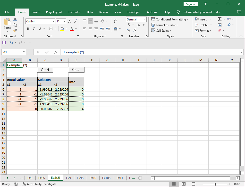
Hybrd1 iteratively computes the closest zero starting from the given initial estimate. This program tests five different initial values to examine the solutions obtained.

First, four initial points corresponding to the expected solutions are tested: (1, 1), (-1, 1), (1, -1), (-1, -1). Additionally, we test (0, 0) to observe its behavior.

Running this program yields the following results:

Each starting point converged to the nearest solution, except when starting from (0, 0), which converged to the upper-left solution.

8.3.2 Solving Using VBA Program (2)

Below is an example using Hybrd1_r, the reverse communication version (RCI).

Sub Start()
    Const NMax = 10
    Dim N As Long, X(NMax) As Double, Fvec(NMax) As Double, XTol As Double
    Dim Info As Long, I As Long
    Dim XX(NMax - 1) As Double, YY(NMax - 1) As Double, IRev As Long
    '--- Initialization
    N = 2
    XTol = 0.000000000001 '1e-12
    For I = 0 To 4
        '--- Input data
        X(0) = Cells(6 + I, 1): X(1) = Cells(6 + I, 2)
        '--- Compute zeros of system of equations
        IRev = 0
        Do
            Call Hybrd1_r(N, X(), Fvec(), XTol, Info, XX(), YY(), IRev)
            If IRev = 1 Or IRev = 2 Then
                YY(0) = 4 * XX(0) ^ 2 + XX(1) ^ 2 - 16
                YY(1) = XX(0) ^ 2 + XX(1) ^ 2 - 9
            End If
        Loop While IRev <> 0
        '--- Output zeros
        Cells(6 + I, 3) = X(0): Cells(6 + I, 4) = X(1): Cells(6 + I, 5) = Info
    Next
End Sub

Instead of using an external function, this version directly computes values when IRev = 1 or 2, assigns them to YY(), and re-calls Hybrd1_r. More details on RCI are available here.

Running this program produces the same results.

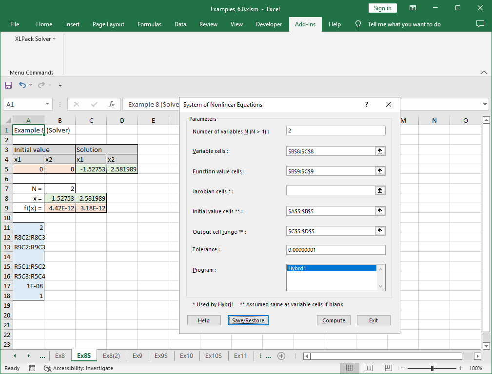
8.3.3 Solving Using the Solver

The XLPack Solver Add-in can also solve the system using the “System of Nonlinear Equations” function. The formulas (=4*B8^2+C8^2-16 and =B8^2+C8^2-9) are entered in cells B9 and C9.

For more information about the solver, refer to this link.

8.3.4 Solving Using VBA Program (3)

Example Problem 2

Modify the previous equation slightly:
\[
\begin{align}
& f_1(x_1, x_2) = 4x_1^2 + (x_2 – 2)^2 – 16 = 0 \\
& f_2(x_1, x_2) = x_1^2 + x_2^2 – 9 = 0 \\
\end{align}
\] The function’s shape now looks as follows:

As seen in the plot, there are now only two solutions instead of four.

Modify the function Sub F() in the previous VBA program:

Sub F(N As Long, X() As Double, Fvec() As Double, IFlag As Long)
    Fvec(0) = 4 * X(0) ^ 2 + (X(1) - 2) ^ 2 - 16
    Fvec(1) = X(0) ^ 2 + X(1) ^ 2 - 9
End Sub

Using the same initial values, the following results were obtained:

The initial values (1, 1) and (-1, 1) converged to nearby solutions. However, the initial values (1, -1) and (-1, -1) unexpectedly converged to distant solutions. And (0, 0) failed to converge and could not find a solution.

If solving fails, check whether the initial value is too far from the root, and whether the equation actually has a real solution.