7. Nonlinear Equations (Single Variable)

7.1 Overview

This section discusses the problem of finding the real-valued zeros of a general single-variable function \(f(x)\):
\[
f(x) = 0
\] If \(f(x)\) is expressed as a polynomial, it is called an algebraic equation, and specialized methods are used to solve it (see Chapter 6).

Otherwise, it is called a nonlinear equation (or transcendental equation). Here, we assume that a real solution exists. Unless an analytical inverse function can be found, an iterative method is used to approximate the solution starting from an initial guess.

7.2 Methods for Solving Nonlinear Equations (Single Variable)

The most common method is Newton’s method, known for its fast convergence, making it widely used in numerical computations. Additionally, a more stable approach is bisection method, which progressively reduces the interval containing the root.

7.2.1 Newton’s Method

Expanding \(f(x)\) around the k-th approximation \(x_k\) using a Taylor series gives the following result.
\[
f(x) = f(x_k) + f'(x_k)(x – x_k) + (1/2)f”(x_k)(x – x_k)^2 + \dots
\] Here, by approximating up to the second term on the right-hand side (assuming terms of second-order and higher are zero) and setting \(f(x) = 0\), the following equation is obtained:
\[
x = x_k – \frac{f(x_k)}{f'(x_k)}
\] Using this \(x\) as the (k + 1)-th approximation \(x_{k+1}\), the following iterative formula for Newton’s method is derived.
\[
\begin{align}
& d_k = -\frac{f(x_k)}{f'(x_k)} \\
& x_{k+1} = x_k + d_k \\
\end{align}
\]

The iteration starts from a suitable initial approximation \(x_0\), and when \(|d_k|\) becomes sufficiently small, it is considered to have converged and the process ends.

The error in the equation is of the order of the square of \(d_k\), and this method is said to exhibit quadratic convergence.

The geometric interpretation of this method is as follows.

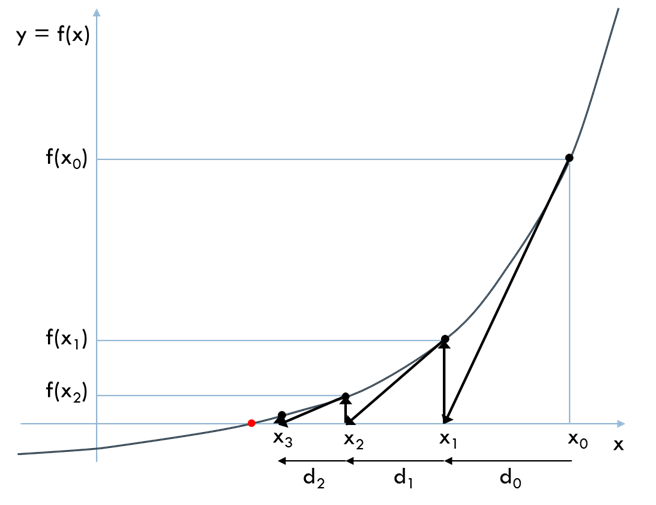
Starting from \(x_0\), the tangent line at that point intersects the \(x\)-axis at \(x_1\). The derivative \(f'(x_0)\) represents the slope of the tangent line, which is used to determine the intersection point \(x_1\).

Similarly, by iteratively finding the next points \(x_2, x_3, \dots\), it can be observed that they rapidly converge to the solution.

This method is widely used due to its rapid convergence. However, it may not be applicable if it is difficult to calculate the derivative \(f'(x)\).

Additionally, it requires an initial value that is sufficiently close to the solution within a region where the function can be considered smooth. Examples of failure due to a poor initial value are as follows.

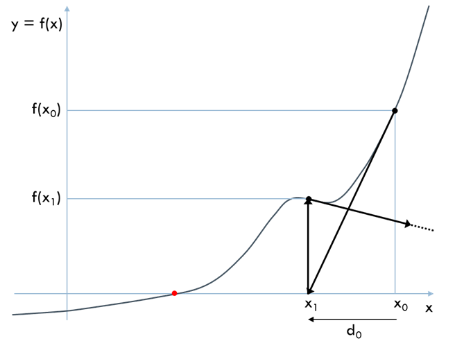
In this example, during the second iteration, divergence occurs (jumping to an unexpected \(x\)). As a result, it may lead to overflow or enter into an infinite loop.

7.2.2 Bisection Method

Two initial points, \(a\) and \(b\), are provided, with function values \(f(a)\) and \(f(b)\). The interval \([a, b]\) must contain only one root. Thus, the signs of \(f(a)\) and \(f(b)\) must be opposite.

The function value \(f(c)\) is calculated at the midpoint \(c = (a + b)/2\).

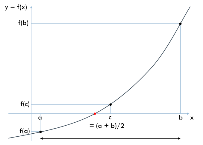
If the sign of \(f(c)\) is the same as that of \(f(a)\), then \(c\) is set as the new \(a\). Otherwise, \(c\) is set as the new \(b\). Then, a new \(c = (a + b)/2\) is calculated, and the process is repeated.

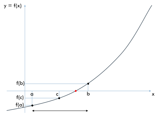
This method, which halves the interval width with each iteration, is called the bisection method. The iteration ends when the interval width becomes sufficiently small.

While this method does not converge quickly, it has the distinct advantage of guaranteed convergence as long as the interval containing the solution is known. Additionally, the absence of the need to calculate derivatives is another benefit.

7.3 Solving Single-Variable Nonlinear Equations Using XLPack

The VBA subroutine Dfzero finds a solution faster than the bisection method when provided with an interval containing a root. During iteration, interpolation is performed using three points \(a, b, and c\) to estimate the zero. If this estimate is reasonable, it is accepted; otherwise, the bisection method is applied. Overall, this method converges faster than standard bisection. Dfzero can also be used via the XLPack solver.

Example Problem

Solve the following equation:
\[
f(x) = x^3 – 2x – 5 = 0
\] To examine the shape of \(f(x)\), let’s plot its graph:

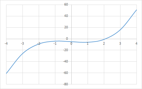
The zero is located near \(x = 2\), so we adopt the interval \([1, 3]\) to enclose the root.

7.3.1 Solving Using VBA Program (1)

Below is a VBA program using Dfzero:

Function F(X As Double) As Double
    F = X ^ 3 - 2 * X - 5
End Function

Sub Start()
    Dim Ax As Double, Bx As Double, Rx As Double, Re As Double, Ae As Double, Info As Long
    '--- Input data
    Ax = 1
    Bx = 3
    Rx = Ax
    Re = 0.000000000000001 '1e-15
    Ae = Re
    '--- Compute zero of equation
    Call Dfzero(AddressOf F, Ax, Bx, Rx, Re, Ae, Info)
    '--- Output zero
    MsgBox Str(Ax) & " (Info = " & Str(Info) & ")"
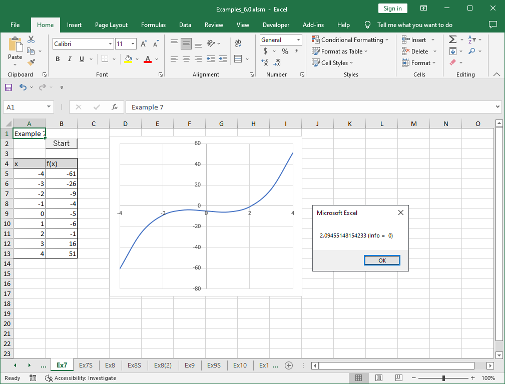
End Sub

An external function defines \(f(x)\), and Dfzero is called with the interval and desired precision.

Care must be taken to provide an interval that definitely contains a zero. If the given interval includes multiple zero points, the specific point to which the method converges is unpredictable.

Executing this program yields \(x = 2.0945514815\).

7.3.2 Solving Using VBA Program (2)

Below is an example program using Dfzero_r, the reverse communication version (RCI).

Sub Start()
    Dim Ax As Double, Bx As Double, Rx As Double, Re As Double, Ae As Double, Info As Long
    Dim XX As Double, YY As Double, IRev As Long
    '--- Input data
    Ax = 1
    Bx = 3
    Rx = Ax
    Re = 0.000000000000001 '1e-15
    Ae = Re
    '--- Compute zero of equation
    IRev = 0
    Do
        Call Dfzero_r(Ax, Bx, Rx, Re, Ae, Info, XX, YY, IRev)
        If IRev <> 0 Then YY = XX ^ 3 - 2 * XX - 5
    Loop While IRev <> 0
    '--- Output zero
    MsgBox Str(Ax) & " (Info = " & Str(Info) & ")"
End Sub

Instead of defining an external function, the reverse communication interface evaluates \(f(x)\) within the loop when IRev = 1, assigning the result to YY, and re-invoking Dfzero_r. More details on RCI are available here.

Running this program produces the same result.

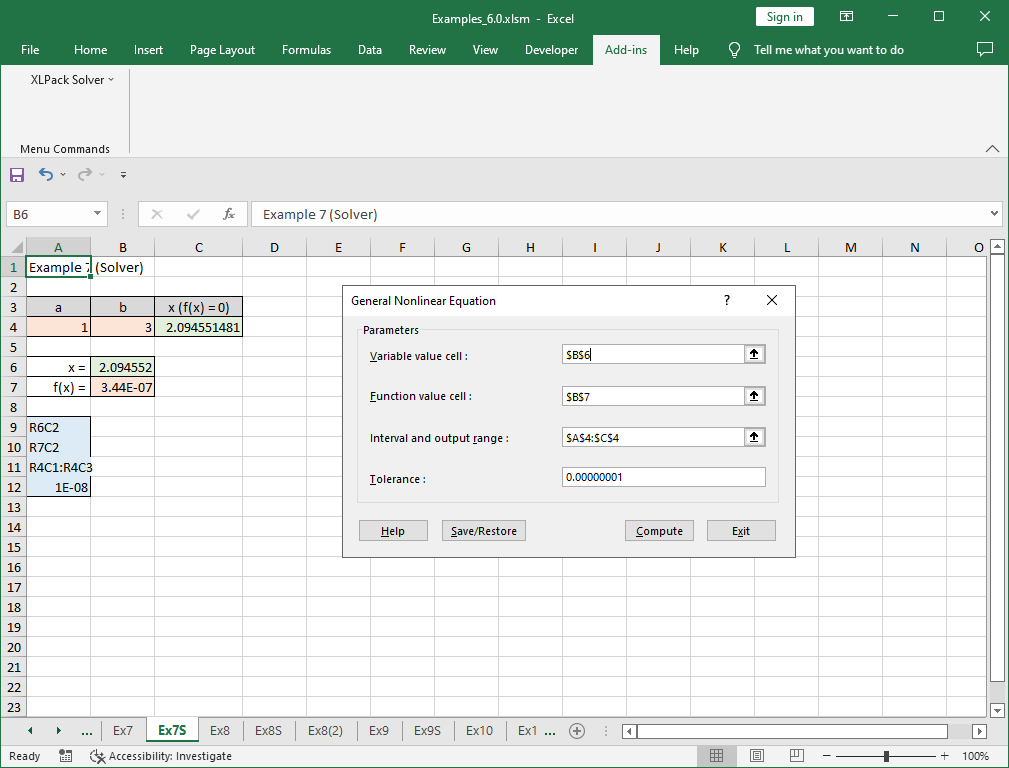
7.3.3 Solving Using the Solver

The XLPack Solver Add-in can also solve the equation using the “General Nonlinear Equation” function. The formula (=B6^3-2*B6-5) is entered in cell B7.

For more information about the solver, refer to this link.